Center of Biomass Conditions
Environmental Conditions at Encounter Locations for Marine Species
Encounter Temperatures of Size-at-Age Species
Species encountering temperature changes may respond to a changing environment in a number of ways. One approach is that species may choose to change location to a more suitable environment. However; this approach may not be an option for all species. Certain species, and individuals of other species, may lack the mobility/awareness needed to relocate and must survive/persist in the new environment.
This document will look at the different temperatures that species have been caught at. Temperatures will be taken from the CTD casts deployed as part of the groundfish survey to take advantage of bottom temperatures.
The general hypothesis follows that species that are better able to track favorable temperatures should experience a lesser physiological toll than species that are unable to track temperature change. Changes in size-at-age should consequently be smaller in highly mobile species than less adaptable ones.
Species Used:
The species used here will match the 16 species included as part of the size-at-age analysis. Those species are:
Code
# Size at age species
saa_species <- c("acadian redfish", "american plaice",
                 "atlantic cod", "atlantic herring",
                 "atlantic mackerel", "black sea bass",
                 "butterfish", "haddock", "pollock", "red hake",
                 "scup", "silver hake", "summer flounder",
                 "white hake", "winter flounder",
                 "witch flounder", "yellowtail flounder")

# table for printing
spec_df <- data.frame("Species" = saa_species)
spec_df %>% knitr::kable()| Species |
|---|
| acadian redfish |
| american plaice |
| atlantic cod |
| atlantic herring |
| atlantic mackerel |
| black sea bass |
| butterfish |
| haddock |
| pollock |
| red hake |
| scup |
| silver hake |
| summer flounder |
| white hake |
| winter flounder |
| witch flounder |
| yellowtail flounder |
Data for these 17 species comes from fisheries independent trawl survey data collected by NOAA and the NEFSC.
Code
# Load the regional temperatures from {targets}
withr::with_dir(rprojroot::find_root('_targets.R'),
                tar_load(nefsc_stratified))

# Filter to just them, and the two time regimes
trawldat <- nefsc_stratified %>%
  filter(comname %in% saa_species)

# Pull the main columns to speed things up
trawldat <- trawldat %>%
  select(cruise6, station, stratum, tow, survey_area,
         svvessel, source, est_year, est_towdate,
         season, decdeg_beglat, decdeg_beglon,
         avgdepth, bottemp, comname, scientific_name,
         abundance, biomass_kg,
         catchsex, sum_weight_kg)


# Set up the regimes
trawldat <- trawldat %>%
  mutate(temp_regime = ifelse(between(est_year, 2000, 2009), "Early Regime", NA),
         temp_regime = ifelse(between(est_year, 2010, 2019), "Warm Regime", temp_regime),
         temp_regime = ifelse(est_year < 2010, "Historical Context", temp_regime))
Code
# Summarize to total biomass per tow:

####  WORKING HERE  ####

# 1. station_totals = biomass and abundance from each tow for all species
# Totals up the abundance and biomass across sex*
station_totals <- trawldat %>%
  group_by(est_year, survey_area, stratum, tow, est_towdate, avgdepth, bottemp, decdeg_beglat, decdeg_beglon, temp_regime, comname) %>%
  summarise(
    biomass_kg = sum(biomass_kg, na.rm = T),
    .groups = "drop")


# 2. yrly_avgs = average and sd of biomass
year_avgs <- station_totals %>%
  group_by(temp_regime, comname, est_year) %>%
  summarise(
    total_biomass   = sum(biomass_kg),
    avg_biomass     = mean(biomass_kg),
    biomass_sd      = sd(biomass_kg),
    avg_depth       = weightedMean(avgdepth, w = biomass_kg, na.rm = T),
    avg_temp        = weightedMean(bottemp, w = biomass_kg, na.rm = T),
    avg_lat         = weightedMean(decdeg_beglat, w = biomass_kg, na.rm = T),
    avg_lon         = weightedMean(decdeg_beglon, w = biomass_kg, na.rm = T),
    depth_sd        = weightedSd(avgdepth, w = biomass_kg, na.rm = T),
    temp_sd         = weightedSd(bottemp, w = biomass_kg, na.rm = T),
    lat_sd          = weightedSd(decdeg_beglat, w = biomass_kg, na.rm = T),
    lon_sd          = weightedSd(decdeg_beglon, w = biomass_kg, na.rm = T),
    .groups = "drop"
  )


# Variance across all years within each species
global_benchmarks <- station_totals %>%
  group_by(comname) %>%
  summarise(
    avg_biomass     = mean(biomass_kg),
    biomass_sd      = sd(biomass_kg),
    avg_depth       = weightedMean(avgdepth, w = biomass_kg, na.rm = T),
    avg_temp        = weightedMean(bottemp, w = biomass_kg, na.rm = T),
    avg_lat         = weightedMean(decdeg_beglat, w = biomass_kg, na.rm = T),
    avg_lon         = weightedMean(decdeg_beglon, w = biomass_kg, na.rm = T),
    depth_sd        = weightedSd(avgdepth, w = biomass_kg, na.rm = T),
    temp_sd         = weightedSd(bottemp, w = biomass_kg, na.rm = T),
    lat_sd          = weightedSd(decdeg_beglat, w = biomass_kg, na.rm = T),
    lon_sd          = weightedSd(decdeg_beglon, w = biomass_kg, na.rm = T),
    .groups = "drop"
  )
Regional surface Temperatures
Using OISST data for the region, and a 30-year climatology, we know that the region has experienced the following trend in sea surface temperature anomalies:
Code
# What were temps doing over the whole region:
oisst_all <- oisst_access_timeseries("nmfs_trawl_regions", poly_name = "inuse strata", mac_os = "mojave")

# Make Yearly averages
oisst_yrs <- oisst_all %>%
  mutate(time = as.Date(time)) %>%
  group_by(year = lubridate::year(time)) %>%
  summarise(
    temp = mean(area_wtd_sst),
    clim = mean(area_wtd_clim),
    anom = mean(area_wtd_anom))# %>%
  #filter(between(year, 2000, 2019))


ggplot(oisst_yrs, aes(year, anom)) +
  geom_line(linetype = 2, size = 0.75) +
  geom_point(size = 2, color = gmri_cols("gmri blue")) +
  labs(title = "Survey Area Temperature Anomalies",
       x = "Year",
       y = "Temperature Anomaly °C")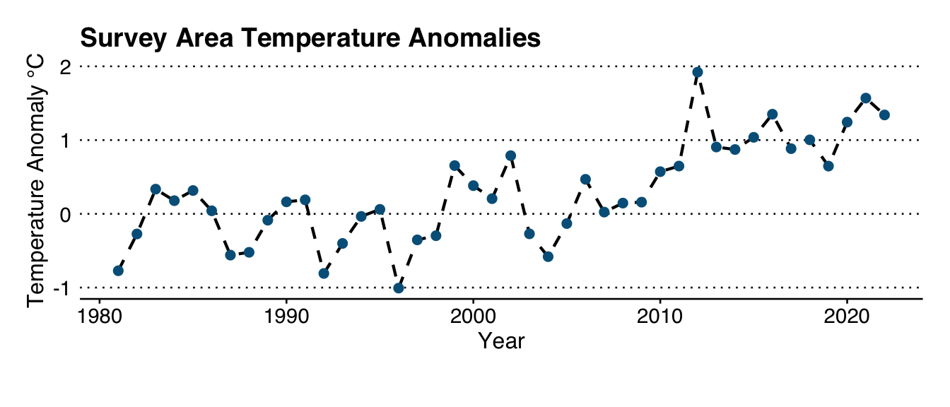
Yearly-Averaged Preferences
The following interactive plots display the biomass weighted averages for what temperatures, depths, and latitudes Each species was caught at as part of the groundfish survey.
Code
# Standardize all the actual measurements
z_data <- map_dfr(saa_species, function(filter_spec){

  glob_metrics <- filter(global_benchmarks, comname == filter_spec)
  year_avgs %>%
    filter(comname == filter_spec) %>%
    mutate(
      depth_z = (avg_depth - glob_metrics$"avg_depth") / glob_metrics$"depth_sd",
      temp_z  = (avg_temp - glob_metrics$"avg_temp") / glob_metrics$"temp_sd",
      lat_z   = (avg_lat - glob_metrics$"avg_lat") / glob_metrics$"lat_sd",
      lon_z   = (avg_lon - glob_metrics$"avg_lon") / glob_metrics$"lon_sd"
    )

})
For anything that is standardized, it is done so against the average value for that species using data from all years.
Code
# Reformat years as a date - messes with slider
# year_avgs <- mutate(year_avgs, est_year = as.Date(str_c(est_year, "-06-01")))

# Define data to use for js
ojs_define(pref_data = z_data)
Now we write the filtering function that will transform the data passed to observable using the values of est_year and comname.
Code
// Filtering Function
filtered = transpose(pref_data).filter(function(trawldat) {
  return year_min < trawldat.est_year &&
         comname.includes(trawldat.comname);
})
To use our filter we’ll need some inputs, and we’ll want to be able to use the values of these inputs in our filtering function. To do this, we use the viewof keyword and with some standard Inputs:
Plot Controls
The following controls will update the data for all plots simultaneously allowing direct comparison across multiple variables and species simultaneously.
Code
viewof year_min = Inputs.range(
  [1970, 2019],
  {value: 1970, step: 1, label: "Starting Year:"}
)

viewof comname = Inputs.checkbox(
  ["acadian redfish", "american plaice",
   "atlantic cod", "atlantic herring",
   "atlantic mackerel", "black sea bass",
   "butterfish", "haddock", "pollock", "red hake",
   "scup", "silver hake", "summer flounder",
   "white hake", "winter flounder",
   "witch flounder", "yellowtail flounder"],
  { value: ["white hake", "black sea bass", "yellowtail flounder", "silver hake"],
    label: "Species:"
  }
)
Finally, we’ll plot the filtered data using Observable Plot (an open-source JavaScript library for quick visualization of tabular data):
Code
Plot.plot({
  style: "overflow: visible;",
  y:{grid : true,
     label: "↑ Latitude (N)"},
  x:{grid : false,
     label: "Year →",
     tickFormat: d3.format(".1d")},
  marks: [
      Plot.line(filtered, {
        x: "est_year",
        y: "avg_lat",
        stroke: "comname",
        marker: "circle"}),
      Plot.text(filtered, Plot.selectLast({
        x: "est_year",
        y: "avg_lat",
        z: "comname",
        text: "comname",
        textAnchor: "start",
        dx: 3
    }))
    ]
  }
)
Code
Plot.plot({
  style: "overflow: visible;",
  y:{grid : true,
     reverse: true,
     label: "↓ Depth (m)"},
  x:{grid : false,
     label: "Year →",
     tickFormat: d3.format(".1d")},
  marks: [
      Plot.line(filtered, {
        x: "est_year",
        y: "avg_depth",
        stroke: "comname",
        marker: "circle"}),
      Plot.text(filtered, Plot.selectLast({
        x: "est_year",
        y: "avg_depth",
        z: "comname",
        text: "comname",
        textAnchor: "start",
        dx: 3
    }))
    ]
  }
)
Code
Plot.plot({
  style: "overflow: visible;",
  y:{grid : true,
     label: "↑ Temperature (C)"},
  x:{grid : false,
     label: "Year →",
     tickFormat: d3.format(".1d")},
  marks: [
      Plot.line(filtered, {
        x: "est_year",
        y: "avg_temp",
        stroke: "comname",
        marker: "circle"}),
      Plot.text(filtered, Plot.selectLast({
        x: "est_year",
        y: "avg_temp",
        z: "comname",
        text: "comname",
        textAnchor: "start",
        dx: 3
    }))
    ]
  }
)
Standardized Shifts:
The following figures all display how a given variable has shifted relative to the overall variance seen for that variable x species. This allows for easier comparison across species.
Code
Plot.plot({
  style: "overflow: visible;",
  y:{grid : true,
     label: "↑ Latitude (z)"},
  x:{grid : false,
     label: "Year →",
     tickFormat: d3.format(".1d")},
  marks: [
      Plot.line(filtered, {
        x: "est_year",
        y: "lat_z",
        stroke: "comname",
        marker: "circle"}),
      Plot.text(filtered, Plot.selectLast({
        x: "est_year",
        y: "lat_z",
        z: "comname",
        text: "comname",
        textAnchor: "start",
        dx: 3
    }))
    ]
  }
)
Code
Plot.plot({
  style: "overflow: visible;",
  y:{grid : true,
     reverse: true,
     label: "↓ Depth (z)"},
  x:{grid : false,
     label: "Year →",
     tickFormat: d3.format(".1d")},
  marks: [
      Plot.line(filtered, {
        x: "est_year",
        y: "depth_z",
        stroke: "comname",
        marker: "circle"}),
      Plot.text(filtered, Plot.selectLast({
        x: "est_year",
        y: "depth_z",
        z: "comname",
        text: "comname",
        textAnchor: "start",
        dx: 3
    }))
    ]
  }
)
Code
Plot.plot({
  style: "overflow: visible;",
  y:{grid : true,
     label: "↑ Temperature (z)"},
  x:{grid : false,
     label: "Year →",
     tickFormat: d3.format(".1d")},
  marks: [
      Plot.line(filtered, {
        x: "est_year",
        y: "temp_z",
        stroke: "comname",
        marker: "circle"}),
      Plot.text(filtered, Plot.selectLast({
        x: "est_year",
        y: "temp_z",
        z: "comname",
        text: "comname",
        textAnchor: "start",
        dx: 3
    }))
    ]
  }
)
Change Pathways
Over the course of several years the mechanism by which a species may seek relief may change. This may be due to some sort of geographical restrictions that may limit the accessibility to deeper water, or some physical barriers that may prevent northward movements.
By displaying how both these axes have shifted through time it may help disclose how a species is moving and during which periods.
Code
path_filtered = transpose(pref_data).filter(function(trawldat) {
  return year_start < trawldat.est_year && species.includes(trawldat.comname);
})

// Species view controls
viewof year_start = Inputs.range(
  [1970, 2019],
  {value: 1990, step: 5, label: "Starting Year:"}
)


viewof species = Inputs.checkbox(
  ["acadian redfish", "american plaice",
   "atlantic cod", "atlantic herring",
   "atlantic mackerel", "black sea bass",
   "butterfish", "haddock", "pollock", "red hake",
   "scup", "silver hake", "summer flounder",
   "white hake", "winter flounder",
   "witch flounder", "yellowtail flounder"],
  { value: ["black sea bass"],
    label: "Species:"
  }
)
Code
Plot.plot({
  style: "overflow: visible;",
  x:{grid : false,
     label: "↑ Latitude (z)"},
  y:{grid : true,
     reverse: true,
     label: "↓ Depth (z)"},
  marks: [
      Plot.line(path_filtered, {
        x: "lat_z",
        y: "depth_z",
        curve: "catmull-rom",
        stroke: "comname",
        marker: "circle"}),
      Plot.text(path_filtered, {
        filter: d => d.est_year % 5 == 0,
        x: "lat_z",
        y: "depth_z",
        z: "est_year",
        text: d => `${d.est_year}`,
        dy: -8
    })
    ],

  // Include a legend for the color channel
  color: {
    legend: true
  }
})