The Northwest Atlantic Ocean is among the fastest warming areas on Earth for sea surface temperature (SST). This region is home to diverse marine ecosystems and supports some of the most valuable fisheries in the United States. The high rate of warming seen over the last decade has scientists concerned that temperatures may outpace the ability of individual species and ecosystems to adjust/acclimate and lead to a decline in ecosystem function. Ecological theory and supporting laboratory studies suggest elevated temperatures are likely to alter body-size across many species by imposing increased metabolic costs at the cellular level and at the individual level through behavior change and altered growth trajectories. However it remains unclear the extent these relationships may be mitigated by the adaptive behaviors of individuals, and how those actions will manifest at the ecological scale in an open-ocean environment. Here we’ve measured ecosystem wide changes in community size spectra, a measure of the community size structure, to track ecosystem functionality in time. We anticipated that where adaptive responses were outpaced by elevated temperatures, the size spectrum slope would steepen, reflecting a decrease in the overall energy transfer efficiency from small to large body sizes. Using fisheries independent survey data we estimated the size spectra relationships for four regions along the US NE continental shelf. Regression analyses were then used to explore how size spectra changes aligned with large-scale, bottom-up, and top-down changes in biotic and abiotic drivers. Spectra slope steepness followed a latitudinal pattern with shallower spectra found in the North and steeper spectra moving South. Changes in slope were most dynamic in the Gulf of Maine, with the other regions showing either gradual change or no change over time. Changes to the Gulf of Maine size structure are most visible among groundfish. These species showed large declines in both average length and average body weight which reflected declining abundance of larger individuals. Gulf of Maine spectra changes can be broken into three periods: a period of steepening from 1982-1998, a brief reversal from 1999-2006, and continued lows after 2006. The largest declines in spectra occurred in the 80’s and 90’s, before the rapid warming of the last decade. Recent lows happening concurrently with both elevated temperatures and declines in primary productivity. Fisheries landings were strongly correlated with these early declines, but that relationship has weakened with time. After 2006 large zooplankton abundances showed strong positive correlations with shallower slopes in the Gulf of Maine, highlighting an important bottom-up influence on the recent size structure. Other regions in this study were less well predicted by changes in fisheries landings and were more impacted by environmental factors. These results highlight the differing vulnerabilities of geographically adjacent marine communities to a common suite of large-scale drivers.
Introduction
Efforts to understand the impacts of climate change at local and regional scales are a high priority area of study among the international scientific community. Concerns about the future health of marine environments have been elevated now that temperature, acidification, sea level, and ocean circulation patterns have all shown signs of recent rapid change (Johnson and Lyman (2020); Findlay and Turley (2021); University of South Carolina et al. (2021); Frederikse et al. (2020); Neto et al. (2021)). Within the context of temperature changes, scientists anticipate ecological communities will respond to rising temperatures through actions to avoid, limit exposure, and/or adapt to unfavorable conditions. At a community-scale, adaptation will ultimately be limited by the constraints of what each constituent species’ life histories can support. Possible pathways for mitigating the impacts of rising temperatures include physical shifts in geographic distributions and depth as well as physiological changes impacting growth and maturation relationships (Atkinson (1995); Blackburn et al. (1999); Pinsky et al. (2013)). When considering ecological responses to warming, a major constraint for adaptation pathways is direct human intervention. Marine ecosystems are tightly coupled to human systems and are shaped by human interactions like fishing and other practices that alter the marine environment in unforeseen ways. These human interactions have been shown to directly alter geographic distribution and life-history features of target and non-target species. This can in turn change the available adaptive pathways and adaptive responses for climate-stressed species (Law (2000); Mills et al. (2013) ; Perälä et al. (2022) ; Rabalais and Turner (2019) ; Tu et al. (2018)). Marine communities are complex and difficult to sample accurately and consistently over large scales. Research on the early impacts of climate change on marine systems has focused on individual species or small communities that can be consistently sampled and/or have their interactions explicitly described (Pinsky et al. (2013) , Nye et al. (2009) , Pershing et al. (2015) ). One weakness in these approaches is the assumptions they rest upon. For many species distribution studies there is an implicit assumption that key ecological interactions will be preserved under projected climate change conditions, that ecosystem function and community structures will be maintained. Another lens with which to study the functionality of a community is through the study of its traits. Size is commonly referenced as the master trait and has well documented relationships to metabolism and community organization (Brown et al. (2000); White et al. (2007)). Marine communities are very-often size-structured, size correlating to trophic position, making them ideal for investigation through this lens. Size spectra relate how the abundance of individuals changes with increasing body size (Sheldon et al. (1972)). In marine systems it has been noted that the summed biomass concentration of individual aquatic organisms is roughly constant across equal logarithmic intervals of body size from bacteria to the largest predators. The rate at which abundance declines with increasing size reflects how well energy is transferred from the smallest individuals at the lowest trophic levels to larger individuals occupying higher trophic levels (Andersen and Beyer (2006) ; Hillaert et al. (2018)). Measuring size spectra is a taxon-agnostic method to detect changes in ecosystem health and has been shown to be sensitive to both large-scale environmental disturbance as well as direct human interaction (Shin et al. (2005); Kerr and Dickie (2001)). By studying changes in energy-transfer efficiency (spectrum slope) scientists can assess the robustness of communities to external stressors and environment change (Sprules and Barth (2016)). Our study focuses on changes in the size structure of the Northeast US continental shelf finfish community. This region is experiencing rapid increases to temperature tied to changes in the behaviors of the Gulf Stream and Labrador Currents (University of South Carolina et al. (2021)). This region has been sampled extensively as part of national fisheries management efforts and has long-term records on the size distribution of the finish community, providing a long-history with which to study changes in size structure. Our study measures size-structure characteristics for the finfish community across four sub-regions (Gulf of Maine, Georges Bank, Southern New England, Mid-Atlantic Bight). These subregions follow a North to South temperature gradient that supports a range of biological communities associated with their distinct temperature regimes. Based on early observational studies and ecological theory we anticipate that individual level responses to a rapidly warming environment will be detectable in the size-structure of the region’s ecological community, evidence that ecosystems are experiencing change-of-function as a result of rapid environmental change. Using the size spectra timeseries for the relative impact of major external drivers we will assess the relative impact of major regional environmental factors.
Methods
Fish Community Data Source and Processing
Abundance, biomass, and size data for Northeast U.S. Shelf fish species were collected as part of the Northeast Fisheries Science Center’s bottom trawl survey (Grosslein 1969, Azarovits 1981, Politis 2014). This survey has been conducted from Cape Hatteras, North Carolina to the Gulf of Maine in the spring and in fall of each year since 1968. The survey follows a stratified random sampling design, with stratum characterized by depth, bottom habitat, and latitude. Tows are performed for a fixed duration at each station. The aggregate abundance and biomass for each species caught is reported, as well as a length measurement for all individuals (sub-samples taken for in cases of a very large catch). Correction factors were applied to abundance and biomass values to account for changes in vessels, gear, and doors used in the survey (Sissenwine and Bowman 1978, Byrne and Forrester 1991, Miller et al. 2010). We performed an additional correction on the individual-level abundance at length information for each species to match the aggregate abundance and biomass corrections done by the science center. 68 finfish species were used in our analyses, representing 98.98% of the finfish biomass caught in the survey. These species were selected on the availability of published weight-at-length relationships (Wigley et al. 2003). Length-weight relationships (Wigley et al. 2003 ) were used to convert length data, available for all individuals, into individual weights. Each species was assigned a functional group based on its life history and geography using the definitions of Hare et al. (2016) . Functional groups included coastal fishes, diadromous fishes, elasmobranchs, groundfish, and pelagic fishes (Table 1). Six species were not included in the original work of Hare et al. 2016, these were assigned to the most relevant functional groups (see Table 1). To account for differences in sampling effort among survey stratum, all abundance information and any associated biomass values were area-stratified. All analyses were performed using these area-stratified estimates using only spring and fall surveys from 1970 to 2019. Analyses were performed for four regions composed of groups of survey-design stratum: Gulf of Maine, Georges Bank, Southern New England, Mid-Atlantic Bight (Figure 1a).
Ecological Indicators
For each region we developed the following time series of ecological indicators:
Annual mean abundance and biomass by functional group
Annual mean length and weight of the aggregate community and for each functional group
Annual estimates of the community size spectrum slope
Total abundance and biomass for each sub-region were calculated for each year using area-stratified abundance and the estimates of weight-at-length from Wigley et al. 2003. This process was repeated for each region and for each of the four functional groups. This gave us longitudinal changes to abundance and biomass for the aggregate community and its functional components. Changes to body size were measured using the average length and weight across all 68 species. Average size estimates were weighted by area-stratified abundance. Average body length (cm) and body weight (kg) was calculated for each region and for each functional group. The data for body size estimates was not truncated using any minimum or maximum size and reflects all available catch data for the 68 species in this study. Long-term trends were determined using linear regression. Annual size spectra were calculated for each region using the extended likelihood method (MLEbin) of Edwards et al. (2020) . This method estimates the exponent of the size spectra (b) for a bounded power law relationship between length-specific abundance and length-estimated biomass. The exponent of this relationship is analogous to slope estimates from normalized biomass spectra methods that employ a linear regression on logarithmic axes Carvalho et al. (2021) . This method has been shown to be the most accurate for estimating the exponent of size spectra when tested against alternative methods ( White et al. (2008) ; Sprules and Barth (2016) ; Edwards et al. (2017) ). Using this method, the size spectra exponent (b) was estimated for each region from 1970 to 2019. A minimum body weight of 1g was used for the lower bound and a maximum biomass of 10 kg was used as an upper bound when estimating the size spectra to account for poor survey catchability at the smallest and largest sizes. This size range retained 97.83% of all the biomass for the 68 species included in this study. Exponents of size spectra (b) were calculated using code modified from the sizeSpectra package (Edwards et al. (2017); Edwards et al. (2020)) and implemented using the R statistical programming language.
Drivers of Spectra Change
Impacts of external factors on spectra slope were explored using multiple regression analyses. Annual variation in regional slope was modeled using measures of large-scale environmental conditions, anthropogenic disturbance, and bottom up resource quality. Environmental drivers were the regional SST anomalies and the Gulf Stream Index (GSI). Global SST data were obtained via NOAA’s Optimum Interpolation SST analysis (OISSTv2), which provides daily SST values at a 0.25° latitude x 0.25° longitude resolution Reynolds et al. (2007) . A daily climatology for every 0.25° pixel in the global data set was created using average daily temperatures spanning the period of 1982-2011. Daily anomalies were then computed as the difference between observed temperatures and the daily climatological average. OISSTv2 data used in these analyses were obtained from the NOAA Physical Sciences Laboratory, Boulder, Colorado, USA from their website. SST anomalies were regionally averaged to produce time series for each of the four survey sub-regions described above (Figure 1a). These were then averaged to within years to form annual time series of SST anomalies. The Gulf Stream index (GSI) quantifies the latitude of the Gulf Stream position based on ocean temperatures at 200 m depth between 55° W and 75° W longitude. The index was obtained from the ecodata package in R (Bastille & Hardison 2018), which supplies GSI data at monthly intervals following the methodology of Pérez-Hernández and Joyce (2014) and Joyce et al. (2019) , using sea level height anomaly data from the Copernicus Marine Environment Monitoring Service. Fishing pressure represents the primary top-down anthropogenic driver in the region, and was investigated using regional commercial landings data. Fishing pressure in the region was measured using state and federal commercial fishing landings. This data was obtained from the Greater Atlantic Regional Fisheries Office (GARFO) for statistical areas that are routinely used for fisheries reporting and management. Individual statistical areas were aggregated into clusters that closely aligned with the trawl survey areas (Figure 1b). Bottom-up ecological interactions were explored using two zooplankton indices. Zooplankton indices were from NOAA Fisheries’ Marine Resources Monitoring, Assessment and Prediction (MARMAP) program and Ecosystem Monitoring (EcoMon) cruises ( Morse et al. (2017) ). Abundance anomalies were computed from the expected abundance on the day of sample collection. The small copepod index is computed by averaging the individual abundance anomalies of Pseudocalanus spp., Centropages hamatus, Centropages typicus, and Temora longicornis. The “large-copepod” anomaly values are the abundance anomaly of Calanus finmarchicus, the largest copepod in the Northeast U.S. region ( Kane (2007) , Kane (2008) ). Anomalies for both large and small zooplankton groups were averaged within ecological production units by the data provider, producing annual timeseries for the Gulf of Maine, Georges Bank, and Mid-Atlantic Bight (NMFS 2023). The zooplankton timeseries for the Mid-Atlantic Bight EPU was used for both the Mid-Atlantic Bight and Southern New England regions in our analyses due to shared geographic overlap. Each of these drivers (climate, primary productivity, fishing) have independently been shown in other works to have measurable impacts on size spectra ( Duplisea and Kerr (1995) ; Blanchard et al. (2005) ; Woodworth-Jefcoats and Wren (2020) ). Our exploratory investigations here are an effort to evaluate which predictors most explain the variance seen in the regional size spectra, and whether those relationships have changed over the study period. To highlight potential cases of non-stationarity, a hallmark of regime-shift dynamics ( Blöcker et al. (2023)) , we explored the temporal structures in the regional spectra using breakpoint analyses. Breakpoint analyses were performed using the envcpt package (Killick et al. 2021). This package applies an automatic model selection process testing support for candidate model structures including constant/piecewise changes to the mean, variance, trends, & autocorrelations and any identified changepoints located using the pruned exact linear time algorithm ( Rikardsen et al. (2004) ). Results from the breakpoint analysis were used to identify whether regional spectra expressed distinct periods of change. In cases where changepoints were identified an additional “regime” term was included to the regression analyses of key drivers. This term allowed for non-linear driver effects across different periods of time. Time-lags on predictors were also evaluated to explore important non-contemporaneous relationships between drivers and size spectra. Important lagged relationships were identified through the use of cross correlation function (CCF) estimates. CCFs were performed for the dependent variable of the size spectra slope with the independent variables of SST, GSI, commercial fisheries landings, and small and large zooplankton indices for annual lags up to 10 years. Significant lags were then included as additional candidate predictors in the multiple regression analysis of spectrum slope changes. Multiple regression models were evaluated independently for each region and their performances using AICc to rank the most parsimonious models.
Results
Abundance and Biomass Changes
Abundance has been gradually increasing on the Northeast Shelf since 1970, accelerating after 2007 to peak levels in 2014. Following that peak, shelf-wide numbers have been in decline (Figure 2). In the Gulf of Maine, fish abundance was relatively low until the 1990’s when it began to steadily rise. Abundance here fell during 2002-2006, but then continued to rise after 2006. Gulf of Maine abundance peaked in 2016 and then declined through 2019. Georges Bank abundance was low from 1970 through 2010. By 2014 abundance had roughly quadrupled, propelled by notable strong recruitment classes of haddock and other groundfish species. After peaking in 2014, abundance soon fell to levels more similar to the 1970-2010. Abundance in Southern New England displayed higher inter-annual variability when compared to both Gulf of Maine and Georges Bank. Abundance began increasing rapidly in 2007, before falling back to earlier levels by the end of the 2010’s. The Mid Atlantic Bight displayed a similar inter-annual variability, but had no major trend in fish abundance. Groundfish species were the dominant functional group driving the abundance and trends in the Gulf of Maine and Georges Bank, contributing more than half the total fish abundance in these regions. The two southern regions showed a more balanced abundance distribution among the five functional groups, with a larger representation of coastal and diadromous species (Figure 2). Shelf-wide biomass has been on the rise since the late-1990’s. Biomass peaked in 2016, and fell for the next three years mirroring the pattern seen in abundance (Figure 2). Shelf biomass was concentrated among two major functional groups, groundfish and elasmobranchs. Groundfish biomass was lowest in the late 80’s and early 90’s, before rebounding in the 2000’s. Elasmobranch biomass increased throughout the study period, with the exception of southern New England (Figure 2). Biomass was higher in the two northern regions, the Gulf of Maine and Georges Bank. The Gulf of Maine followed a similar trend to the shelf as a whole. Biomass here was at its lowest during the 1980’s, but had more than doubled by 2000 and in years following, peaking in 2016 before declining each year after. The majority of the biomass here was found among groundfish and elasmobranch species. Georges Bank had a similar groundfish and elasmobranch composition. Biomass here was lowest in the early 1970’s. During the 1980’s groundfish biomass declined, but this was offset by growth in elasmobranch species. The region hit low biomass levels again in the 1990’s before climbing to peak levels in 2014. Biomass then fell here each year after. .In Southern New England the biomass changes were less steady. Increases in the 1980’s were followed by abrupt declines in the mid 1990’s. The region saw its highest biomass in 2012, with a familiar decline towards the end of the timeseries. Biomass here was represented with a majority role of elasmobranch species. This was also the case in the Mid-Atlantic Bight, a region that saw long term growth in its biomass and a peak in 2019.
Northeast shelf length and weight of the “average” individual fish has remained relatively stable over nearly five decades (Figure 2.). Average length did not change over the study, averaging 26.06 cm (sd = 2.57). Average weight declined slowly at 8.95g year-1 of the same period.Independent trends were found within the regional communities. Fish size declines in the Gulf of Maine were the most of any region. Average length was highest in the 1970s & 1980s at around 34.7-34.8 cm, lengths fell to 28 cm in the last decade with an overall trend of -.19 cm year-1 . The average weight also fell during the 1980s, from an average of 0.8 kg in the 1970s to 0.3 kg in the 2010s, a decline of 62.5% and a long-term rate of -1.1g year-1 . Georges Bank average sizes declined in average weight (-5.48g year-1), but with no overall change in length. Declining sizes for both the Gulf of Maine and Georges Bank slowed during the late 2000s, but then continued to fall the following decade. Average body size in southern New England was relatively constant, with no long-term changes in length or weight. The Mid-Atlantic Bight region was the only area with long-term increases in both length (.26cm year-1) and weight (4.89g year-1) during the study period.
Spectra Trend Structure and Lagged Driver Exploration
Breakpoint exploratory analysis showed support for breakpoints in one region, the Gulf of Maine. Slope breakpoints were found in 1998 & 2007 where trends reversed direction, with an additional 2-year autocorrelation also supported. This structure would divide the changes to Gulf of Maine size structure into three periods: 1972-1998, 1999-2006, and 2007-2019. Changes in Georges Bank slope changes were best represented by a single trend structure, with slopes steepening over time. The reverse was the case for the Mid-Atlantic Bight, with slopes becoming more shallow with time. In Southern New England a single mean (intercept) model best reflected the lack of change. Based on these exploratory results, three regime periods were added to the Gulf of Maine multiple regression analysis. A two-year autocorrelation term was also included based on its support in the most parsimonious breakpoint model. No breakpoints or autocorrelation terms were added to the models for the remaining regions. CCF estimates of lagged drivers flagged several relationships in Georges Bank and the Mid-Atlantic Bight. The lagged predictors added to Georges Bank regression models included: A 2-year lag on the small zooplankton index, a 1-year lag on the large zooplankton index, a 1-year lag of SST, 4- & 1-year lags of the GSI, and 4- & 5-year lags of commercial landings. The lagged predictors added to Mid-Atlantic Bight regression models were: 5- & 7-year lags on the small zooplankton index and a 2-year lag on SST.
CCF Results
Size Spectra Slopes
Regional differences in size spectra slopes (b) followed a North to South gradient with shallower spectra in the North and steeper spectra in the South (Figure 4). Northeast shelf slopes were centered around a value of -1 and showed no long-term trends. The Gulf of Maine had the shallowest slope of all regions. This was particularly true in the 1970s and 1980s when spectra slopes were around -0.85 & -0.88. Slopes began declining in the 1980s and continued to steepen through the 1990s. During the early 2000s there was a reversal of this trend, but by 2010 they had begun to steepen again. Gulf of Maine spectra slope estimates remained below -0.9 for most of the last decade putting it in line with the more southern regions. Georges Bank slope values also declined over the study with the largest declines happening over the last decade. Southern New England and Mid-Atlantic Bight slope estimates were steeper than in the northern regions. Southern New England’s spectra slopes showed no long-term change over the study period. The Mid-Atlantic Bight was unique in having slopes that became less steep over the study period, ending shallower than all areas except the Gulf of Maine.
Model rankings using AICc & delta-AICc (Table 1) for the Gulf of Maine best support a regression model containing two predictors with a constant (stationary) effect across all years, and two predictors whose effects across were allowed to vary across the regime periods identified by the changepoint analysis (non-stationary effects). The two constant-effect drivers each had a negative impact on spectra slope. They were the small zooplankton index (p = 0.011) and the two-year autocorrelation term (p = 0.033). Main effects for the regime periods themselves were not significant, highlighting important crossover effects. The inclusion of year-block interactions of the three regimes (1982-1998, 1999-2006, & 2007-2019) with both the commercial landings index and the large zooplankton index allowed these drivers to differently impact size spectrum slope between periods. During the first regime the effect of commercial landings was positive (p = 0.009), but for 1999-2006 the relationship was negative (p = 0.032). During the third regime there was no relationship between commercial landings and spectra changes (p = 0.088). For the large zooplankton index there was no relationship during either of the first two regimes (p = 0.2, p = >0.9). During the third regime large zooplankton had a positive effect on the spectrum slope (p = <0.001). For Georges Bank the top performing models (delta-AIC range of <2), four of the five retained two predictors: SST anomalies (p = 0.028) and the small zooplankton index from 2-years prior (p = 0.006). Both of these predictors shared a negative effect on size spectrum slope. A fifth model swapped out SST anomalies for the gulf stream index, again with a negative relationship to spectra slopes. Regression models here highlighted bottom-up drivers as the best predictors, suggesting that this region’s size spectra changes are most highly correlated with environmental forces and not commercial landings. Southern New-England showed no trend in size spectrum slopes. This was further confirmed by the model selection procedure. The “best” model of Southern New England retained only commercial landings, however this relationship was not significant (p = 0.13) and had very low performance (r-squared = 0.06). Three models were selected for the Mid-Atlantic Bight region. The best performing model showed that increases in the small zooplankton index had a negative effect on spectrum slope (p = 0.020). This relationship was present in the other top candidates, with an additional negative relationship with either the large zooplankton or with commercial landings. Model performance was low among the top models (adjusted r-squared 0.14-0.16).
With the rise of ecosystem-based fisheries management practices, size spectrum approaches and size-based indicators have grown in popularity for their ability to reveal system-level properties without the need for explicit parameterization of predator-prey relationships ( Greenstreet et al. (2011) ; Houle et al. (2012) ). This study notes the size structure changes for a community of 68 marine finfish species and spanning four orders of magnitude in body-weight. For the Northeast US shelf as a whole the multi-species size spectra for the has been relatively stable over the last 50 years with values around -1. This is consistent with other large-scale marine studies that measured normalized biomass spectra (Platt & Denman 1977, Quinones et al. (2003) ) and the foundational pattern first documented by Sheldon and subsequently by others ( Sheldon et al. (1972) ; Sprules and Barth (2016) ). We take this as evidence in-tact ecological functionality (as evidenced by the size spectra slope) at this broad geographic scale. While size spectra stability in the Northeast shelf give evidence that these communities have thus far proved resilient to external stress, they may also mask how differently vulnerable these shifting communities are to those same stressors. At regional scales we observed independent size structure trends that highlight differences in the regional responses to disturbance. We observed steady long-term trends in spectra slopes in three regions. These were the steepening in Georges Bank, the shallowing of spectra in the Mid-Atlantic Bight, and a flat trend within Southern New England. These three regions each exhibit spectra near the shelf-wide estimate of -1. Regression driver analyses for these steady-trend areas highlighted bottom-up drivers of small zooplankton, SST anomalies, and the Gulf-Stream index as more informative drivers than measures of fishing pressure. Fisheries are often described as a larger factor on spectra slope steepening, making this result a surprise. However; variance explained for these regional models was low (< .33), a sign that other un-observed or unmeasured factors may be more important or that changes may not be beyond expected natural fluctuation. The most dynamic changes in biomass spectra were observed in the Gulf of Maine, which was viewed across three distinct periods of behavior. In the first period slopes steepened following a decline in abundance of larger individuals primarily composed of groundfish species, a signature consistent with patterns of fishing exploitation seen in other regions ( Duplisea and Kerr (1995) , Rice & Gislaison 1996; Bianchi et al. (2000) ; Jennings and Blanchard (2004) ). Slope estimates during this period were at the time the shallowest of all regions measured, with spectra slope values notably less steep than the broader shelf-wide community >0.9. Following this period commercial landings (a proxy for fishing pressures) remained low for the remainder of the study period, setting hopes for a recovery. During the 1999-2006 period slope steepness had reversed course and became shallower, but after 2006 they then fell again to levels similar to the southern regions. The ultimate failure of the size-structure to recover, despite a release from fishing stress, highlights the challenge managers face in efforts to recover exploited populations. Our analysis suggests that the influence of prey quality in the Gulf of Maine, mainly large or small zooplankton community indices, may help explain how such shallow slopes during the early period were supported, and why slopes remain relatively steep despite a cessation in fishing. A situation likely made worse by the overall declining productivity in the region (Balch et al. 2022). Dynamic food-web models suggest that size-structure recovery can take decades depending on the severity of fishing disturbance ( Fung et al. (2013) ). This has been supported by empirical observations in other regions (Frank et al. 2011; Fogarty and Murawski (1998) ; Daan et al. (2005) ; Hutchings and Reynolds (2004) ; Choi et al. (2004) ). The changing relationships between spectra slope response to large-scale drivers suggest that the vulnerability communities to external factors may shift depending on system state, the level of disturbance, and underlying species composition. While the direct effects of fishing on spectra steepening are perhaps most obvious: removal of larger individuals steepening slope and the out-sized impact their removal has on reduced reproductive output ( Andersen and Rice (2010) ; Law (2000) ; Bianchi et al. (2000) ). The persistence of shallow spectra in periods of reduced fishing is better explained by the less obvious indirect pathways which reinforce size structure imbalances. These include the release of smaller size classes from predation pressure, preserving more biomass at one end of the size spectrum and creating opportunities for diffuse replacement by non-targeted species (Pimm & Hyman 1987; Duplisea and Kerr (1995) ). This can lead to increased competition among the smaller size classes which itself then results in a reduction in adult sizes ( Andersen and Rice (2010) ). A pattern observed in Celtic Sea haddock and here within the Gulf of Maine (Shephard et al 2012). Reduced adult size in adult size stemming from . While it is understood that fishing has large direct and indirect impacts on size spectra, climate impacts have also been shown to impact community size structure ( Blanchard et al. (2005) ). However these impacts are often through other indirect mechanisms, often operating at different time scales ( Blanchard et al. (2005) ; Pershing et al. (2015) ). As size structures become more weighted towards smaller individuals, size structure variability becomes more tightly linked to the abundance and quality of the lower trophic level prey (Shephard et al. 2012). The observation that communities have shifted their size structures toward higher abundances of smaller individuals and lower abundances of larger individuals has been seen across numerous marine systems ( Daan et al. (2005) ; Bianchi et al. (2000) ; Krumsick and Fisher (2020)) . Adding to the challenge already facing natural resource managers is the multi-faceted nature of changing climate. Changes in the distribution and composition of species in our study area have already been reported with an expectation that they will continue and worsen (Friedland et al 2023; Nye et al. (2009)). These factors also likely contribute to size structuring we have seen over the last decade. Empirical size spectra and other size based indicators have grown in popularity with the push for ecosystem based fisheries management practices. They have been shown to be sensitive to the direct human influence of fishing and indirect processes stemming from climate variability. While these taxon-agnostic methods are useful for adding broader context on ecosystem dynamics it can be difficult to isolate the forces driving observed variability. Understanding their limitations, and supporting these methods with complimentary metrics that add to their explainability or allow comparison to an unexploited benchmark should be done as a best practice when possible ( Blanchard et al. (2009) ; Greenstreet et al. (2011) ).
Our study shows that despite a history of large-scale anthropogenic disturbance and a rapidly changing regional climate, changes to the overall community size structure have been minor at broad geographic scales. The regional responses seen appear to operate at different time scales and to different features of the environment. This suggests that at large scales the impacts of a rapidly changing climate may be offset through novel species interactions and an ever-shuffling series of species replacement in a rich biological community. At more local scales we expect breakdowns in these relationships to be more apparent, highlighting the importance of determining the scale of processes involved.
Common and scientific names for the species that constitute each
functional group used in our analyses. X markers are used to indicate
which regions each species has been caught in the data.
Functional Group Assignments and Regional Presence/Absence
Common Name
Scientific Name
Georges Bank
Gulf of Maine
Mid-Atlantic Bight
Southern New England
Coastal - (18)
Atlantic Croaker
micropogonias undulatus
X
X
X
Atlantic Spadefish
chaetodipterus faber
X
Atlantic Thread Herring
opisthonema oglinum
X
X
Black Sea Bass
centropristis striata
X
X
X
X
Blackbelly Rosefish
helicolenus dactylopterus
X
X
X
X
Blueback Herring
alosa aestivalis
X
X
X
X
Bluefish
pomatomus saltatrix
X
X
X
X
Butterfish
peprilus triacanthus
X
X
X
X
Cunner
tautogolabrus adspersus
X
X
X
X
Greater Amberjack
seriola dumerili
X
X
Northern Kingfish
menticirrhus saxatilis
X
X
X
Scup
stenotomus caprinus
X
X
X
X
Southern Kingfish
menticirrhus americanus
X
Spanish Mackerel
scomberomorus maculatus
X
Spanish Sardine
sardinella aurita
X
Spot
leiostomus xanthurus
X
X
Striped Bass
morone saxatilis
X
X
X
X
Weakfish
cynoscion regalis
X
X
X
Diadromous - (2)
American Shad
alosa sapidissima
X
X
X
X
Atlantic Sturgeon
acipenser oxyrhynchus
X
Elasmobranch - (19)
Atlantic Angel Shark
squatina dumeril
X
Atlantic Sharpnose Shark
rhizoprionodon terraenovae
X
Barndoor Skate
dipturus laevis
X
X
X
X
Bullnose Ray
myliobatis freminvillei
X
X
Chain Dogfish
scyliorhinus retifer
X
X
X
Clearnose Skate
raja eglanteria
X
X
Cownose Ray
rhinoptera bonasus
X
Little Skate
leucoraja erinacea
X
X
X
X
Rosette Skate
leucoraja garmani
X
X
X
X
Roughtail Stingray
dasyatis centroura
X
Sand Tiger
carcharias taurus
X
Sandbar Shark
carcharhinus plumbeus
X
X
Smooth Butterfly Ray
gymnura micrura
X
Smooth Dogfish
mustelus canis
X
X
X
X
Smooth Skate
malacoraja senta
X
X
X
X
Spiny Butterfly Ray
gymnura altavela
X
Spiny Dogfish
squalus acanthias
X
X
X
X
Thorny Skate
amblyraja radiata
X
X
X
X
Winter Skate
leucoraja ocellata
X
X
X
X
Groundfish - (25)
Acadian Redfish
sebastes fasciatus
X
X
X
X
American Plaice
hippoglossoides platessoides
X
X
X
X
Atlantic Cod
gadus morhua
X
X
X
X
Atlantic Halibut
hippoglossus hippoglossus
X
X
X
Atlantic Wolffish
anarhichas lupus
X
X
X
Cusk
brosme brosme
X
X
X
X
Fawn Cusk-Eel
lepophidium profundorum
X
X
X
X
Fourspot Flounder
paralichthys oblongus
X
X
X
X
Goosefish
lophius americanus
X
X
X
X
Haddock
melanogrammus aeglefinus
X
X
X
X
Longhorn Sculpin
myoxocephalus octodecemspinosus
X
X
X
X
Northern Searobin
prionotus carolinus
X
X
X
X
Ocean Pout
macrozoarces americanus
X
X
X
X
Offshore Hake
merluccius albidus
X
X
X
X
Pollock
pollachius virens
X
X
X
X
Red Hake
urophycis chuss
X
X
X
X
Sea Raven
hemitripterus americanus
X
X
X
X
Silver Hake
merluccius bilinearis
X
X
X
X
Spotted Hake
urophycis regia
X
X
X
X
Summer Flounder
paralichthys dentatus
X
X
X
X
White Hake
urophycis tenuis
X
X
X
X
Windowpane Flounder
scophthalmus aquosus
X
X
X
X
Winter Flounder
pseudopleuronectes americanus
X
X
X
X
Witch Flounder
glyptocephalus cynoglossus
X
X
X
X
Yellowtail Flounder
limanda ferruginea
X
X
X
X
Pelagic - (4)
Atlantic Herring
clupea harengus
X
X
X
X
Atlantic Mackerel
scomber scombrus
X
X
X
X
Buckler Dory
zenopsis conchifera
X
X
X
X
Round Herring
etrumeus teres
X
X
X
X
Functional group assignments adapted from Hare et al. 2010
Top Commercial Fisheries Landings of Northeastern US (by weight)
Avg. Annual Landings (lb.)
Total Landings (lb.)
Total Value ($)
Gulf of Maine - 1960
Hake, Silver
16.58M
281.87M
8.71M
Herring, Atlantic
11.57M
138.83M
2.50M
Redfish, Acadian
2.12M
88.97M
3.41M
Gulf of Maine - 1970
Herring, Atlantic
22.78M
501.08M
19.70M
Menhaden, Atlantic
17.78M
373.48M
7.87M
Redfish, Acadian
3.14M
219.85M
23.87M
Gulf of Maine - 1980
Herring, Atlantic
21.78M
653.26M
34.52M
Menhaden, Atlantic
21.24M
509.75M
12.77M
Pollock
3.33M
229.57M
62.00M
Gulf of Maine - 1990
Herring, Atlantic
25.21M
958.12M
54.12M
Cod, Atlantic
2.35M
138.76M
131.76M
Shark, Dogfish, Spiny
3.34M
120.17M
15.95M
Gulf of Maine - 2000
Herring, Atlantic
2.99M
47.77M
4.31M
Monkfish/Angler/Goosefish
716.21K
31.51M
51.13M
Cod, Atlantic
692.95K
30.49M
42.30M
Gulf of Maine - 2010
Tuna, Bluefin
209.06K
3.76M
33.30M
Shark, Dogfish, Spiny
479.11K
2.87M
590.62K
Pollock
188.20K
1.69M
2.08M
Georges Bank - 1960
Haddock
15.00M
270.06M
34.41M
Hake, Silver
6.83M
95.57M
3.19M
Cod, Atlantic
4.88M
87.89M
8.12M
Georges Bank - 1970
Cod, Atlantic
7.78M
233.48M
59.16M
Flounder, Yellowtail
4.62M
138.52M
43.16M
Redfish, Acadian
2.63M
76.37M
9.09M
Georges Bank - 1980
Cod, Atlantic
10.11M
404.40M
211.60M
Flounder, Winter
2.50M
100.11M
89.84M
Haddock
2.36M
94.27M
66.68M
Georges Bank - 1990
Cod, Atlantic
4.27M
192.29M
190.26M
Hake, Silver
1.79M
76.82M
20.49M
Flounder, Winter
1.23M
56.43M
75.59M
Georges Bank - 2000
Cod, Atlantic
2.17M
62.91M
75.20M
Herring, Atlantic
3.49M
48.92M
3.73M
Haddock
1.54M
43.01M
55.37M
Georges Bank - 2010
Hake, Silver
155.88K
779.40K
499.90K
Haddock
39.65K
118.95K
143.04K
Flounder, Winter
40.40K
80.80K
216.28K
Southern New England - 1960
Other Fish, Bony
14.84M
400.77M
3.73M
Flounder, Yellowtail
6.56M
196.83M
19.12M
Flounder, Winter
2.52M
70.58M
7.01M
Southern New England - 1970
Menhaden, Atlantic
9.99M
239.84M
5.12M
Other Fish, Bony
4.05M
206.59M
2.49M
Flounder, Yellowtail
2.07M
153.55M
36.47M
Southern New England - 1980
Menhaden, Atlantic
6.60M
217.68M
10.21M
Hake, Silver
2.56M
205.02M
46.11M
Flounder, Yellowtail
1.66M
132.92M
83.38M
Southern New England - 1990
Hake, Silver
2.52M
196.81M
78.54M
Herring, Atlantic
2.12M
129.02M
7.19M
Menhaden, Atlantic
3.71M
125.98M
8.69M
Southern New England - 2000
Mackerel, Atlantic
2.55M
135.06M
15.60M
Hake, Silver
1.00M
55.25M
26.89M
Skate, Nk
950.56K
49.43M
6.53M
Southern New England - 2010
Scup
161.10K
6.44M
4.29M
Hake, Silver
145.07K
4.21M
3.12M
Flounder, Summer
80.43K
3.86M
11.54M
Mid-Atlantic Bight - 1960
Flounder, Summer
2.03K
4.05K
720.00
Flounder, Yellowtail
2.33K
2.33K
214.00
Flounder, Witch
395.00
395.00
36.00
Mid-Atlantic Bight - 1970
Menhaden, Atlantic
10.20M
50.98M
1.59M
Weakfish/Sea Trout, Squeteague
886.91K
9.76M
1.40M
Scup
876.60K
8.77M
2.09M
Mid-Atlantic Bight - 1980
Menhaden, Atlantic
30.78M
646.41M
10.94M
Flounder, Summer
1.15M
83.83M
72.00M
Scup
550.89K
37.46M
15.53M
Mid-Atlantic Bight - 1990
Menhaden, Atlantic
115.86M
4.63B
286.14M
Mackerel, Atlantic
1.67M
103.62M
13.87M
Croaker, Atlantic
1.35M
71.65M
22.53M
Mid-Atlantic Bight - 2000
Menhaden, Atlantic
69.60M
2.64B
167.17M
Croaker, Atlantic
2.16M
106.02M
42.93M
Mackerel, Atlantic
1.70M
59.41M
6.38M
Mid-Atlantic Bight - 2010
Menhaden, Atlantic
118.29M
1.89B
154.46M
Bass, Striped
1.70M
25.56M
75.05M
Croaker, Atlantic
1.08M
24.81M
21.37M
Landings data obtained from the Greater Atlantic Regional Fishing Office (GARFO)
Andersen, K. H., and Rice, J. C. 2010. Direct and indirect community effects of rebuilding plans. ICES Journal of Marine Science, 67: 1980–1988. https://doi.org/10.1093/icesjms/fsq035.
Bianchi, G., Gislason, H., Graham, K., Hill, L., Jin, X., Koranteng, K., Manickchand-Heileman, S., et al. 2000. Impact of fishing on size composition and diversity of demersal fish communities. ICES Journal of Marine Science, 57: 558–571. https://doi.org/10.1006/jmsc.2000.0727.
Blackburn, T. M., Gaston, K. J., and Loder, N. 1999. Geographic gradients in body size: a clarification of Bergmann’s rule. BIODIVERSITY RESEARCH. Diversity <html_ent glyph="@amp;" ascii="&"/> Distributions, 5: 165–174. http://dx.doi.org/10.1046/j.1472-4642.1999.00046.x.
Blanchard, J. L., Dulvy, N. K., Jennings, S., Ellis, J. R., Pinnegar, J. K., Tidd, A., and Kell, L. T. 2005. Do climate and fishing influence size-based indicators of Celtic Sea fish community structure? ICES Journal of Marine Science, 62: 405–411. https://academic.oup.com/icesjms/article/62/3/405/661410.
Blanchard, J. L., Jennings, S., Law, R., Castle, M. D., McCloghrie, P., Rochet, M.-J., and Benoît, E. 2009. How does abundance scale with body size in coupled size-structured food webs? Journal of Animal Ecology, 78: 270–280. https://onlinelibrary.wiley.com/doi/abs/10.1111/j.1365-2656.2008.01466.x.
Blöcker, A. M., Gutte, H. M., Bender, R. L., Otto, S. A., Sguotti, C., and Möllmann, C. 2023. Regime shift dynamics, tipping points and the success of fisheries management. Scientific Reports, 13: 289. https://www.nature.com/articles/s41598-022-27104-y.
Brown, J., West, G. B., and Enquist, B. 2000. Scaling in biology: Patterns and processes, causes and consequences. In pp. 1–24.
Carvalho, P. G., Setiawan, F., Fahlevy, K., Subhan, B., Madduppa, H., Zhu, G., and Humphries, A. T. 2021. Fishing and habitat condition differentially affect size spectra slopes of coral reef fishes. Ecological Applications, 31: e02345. https://onlinelibrary.wiley.com/doi/abs/10.1002/eap.2345.
Choi, J. S., Frank, K. T., Leggett, W. C., and Drinkwater, K. 2004. Transition to an alternate state in a continental shelf ecosystem. Canadian Journal of Fisheries and Aquatic Sciences, 61: 505–510. https://cdnsciencepub.com/doi/abs/10.1139/f04-079.
Daan, N., Gislason, H., G. Pope, J., and C. Rice, J. 2005. Changes in the North Sea fish community: evidence of indirect effects of fishing? ICES Journal of Marine Science, 62: 177–188. https://academic.oup.com/icesjms/article/62/2/177/602590.
Edwards, A., Robinson, J., Blanchard, J., Baum, J., and Plank, M. 2020. Accounting for the bin structure of data removes bias when fitting size spectra. Marine Ecology Progress Series, 636: 19–33. https://www.int-res.com/abstracts/meps/v636/p19-33/.
Frederikse, T., Landerer, F., Caron, L., Adhikari, S., Parkes, D., Humphrey, V. W., Dangendorf, S., et al. 2020. The causes of sea-level rise since 1900. Nature, 584: 393–397. http://dx.doi.org/10.1038/s41586-020-2591-3.
Fung, T., Farnsworth, K., Shephard, S., Reid, D., and Rossberg, A. 2013. Why the size structure of marine communities can require decades to recover from fishing. Marine Ecology Progress Series, 484: 155–171. http://www.int-res.com/abstracts/meps/v484/p155-171/.
Greenstreet, S. P. R., Rogers, S. I., Rice, J. C., Piet, G. J., Guirey, E. J., Fraser, H. M., and Fryer, R. J. 2011. Development of the EcoQO for the north sea fish community. ICES Journal of Marine Science, 68: 1–11. https://doi.org/10.1093/icesjms/fsq156.
Hare, J. A., Morrison, W. E., Nelson, M. W., Stachura, M. M., Teeters, E. J., Griffis, R. B., Alexander, M. A., et al. 2016. A Vulnerability Assessment of Fish and Invertebrates to Climate Change on the Northeast U.S. Continental Shelf. PLOS ONE, 11: e0146756. https://dx.plos.org/10.1371/journal.pone.0146756.
Hillaert, J., Hovestadt, T., Vandegehuchte, M. L., and Bonte, D. 2018. Size-dependent movement explains why bigger is better in fragmented landscapes. Ecology and Evolution, 8: 10754–10767. https://www.ncbi.nlm.nih.gov/pmc/articles/PMC6262741/.
Houle, Jennifer E., Farnsworth, Keith D., Rossberg, Axel G., and Reid, David G. 2012. Assessing the sensitivity and specificity of fish community indicators to management action. Canadian Journal of Fisheries and Aquatic Sciences, 69: 1065–1079. http://www.nrcresearchpress.com/doi/10.1139/f2012-044.
Joyce, T. M., Kwon, Y.-O., Seo, H., and Ummenhofer, C. C. 2019. Meridional Gulf Stream Shifts Can Influence Wintertime Variability in the North Atlantic Storm Track and Greenland Blocking. Geophysical Research Letters, 46: 1702–1708. https://onlinelibrary.wiley.com/doi/abs/10.1029/2018GL081087.
Kane, J. 2007. Zooplankton abundance trends on georges bank, 19772004. ICES Journal of Marine Science, 64: 909–919. https://doi.org/10.1093/icesjms/fsm066.
Kerr, S. R., and Dickie, L. M. 2001. The Biomass Spectrum: A Predator-Prey Theory of Aquatic Production. Columbia University Press.
Krumsick, K. J., and Fisher, J. A. D. 2020. Community size spectra provide indicators of ecosystem recovery on the Newfoundland and Labrador shelf. Marine Ecology Progress Series, 635: 123–137. https://www.int-res.com/abstracts/meps/v635/p123-137/.
Morse, R. E., Friedland, K. D., Tommasi, D., Stock, C., and Nye, J. 2017. Distinct zooplankton regime shift patterns across ecoregions of the u.s. Northeast continental shelf large marine ecosystem. Journal of Marine Systems, 165: 77–91. https://www.sciencedirect.com/science/article/pii/S0924796316303098.
Neto, A. G., Langan, J. A., and Palter, J. B. 2021. Changes in the Gulf Stream preceded rapid warming of the Northwest Atlantic Shelf. Communications Earth & Environment, 2: 1–10. https://www.nature.com/articles/s43247-021-00143-5.
Nye, J., Link, J., Hare, J., and Overholtz, W. 2009. Changing spatial distribution of fish stocks in relation to climate and population size on the Northeast United States continental shelf. Marine Ecology Progress Series, 393: 111–129. http://www.int-res.com/abstracts/meps/v393/p111-129/.
Pershing, A. J., Alexander, M. A., Hernandez, C. M., Kerr, L. A., Le Bris, A., Mills, K. E., Nye, J. A., et al. 2015. Slow adaptation in the face of rapid warming leads to collapse of the gulf of maine cod fishery. Science, 350: 809–812. https://www.science.org/doi/full/10.1126/science.aac9819.
Shin, Y.-J., Rochet, M.-J., Jennings, S., Field, J. G., and Gislason, H. 2005. Using size-based indicators to evaluate the ecosystem effects of fishing. ICES Journal of Marine Science, 62: 384–396. https://doi.org/10.1016/j.icesjms.2005.01.004.
Sprules, W. G., and Barth, L. E. 2016. Surfing the biomass size spectrum: some remarks on history, theory, and application. Canadian Journal of Fisheries and Aquatic Sciences, 73: 477–495. http://www.nrcresearchpress.com/doi/10.1139/cjfas-2015-0115.
Tu, C.-Y., Chen, K.-T., and Hsieh, C. 2018. Fishing and temperature effects on the size structure of exploited fish stocks. Scientific Reports, 8: 7132. https://www.nature.com/articles/s41598-018-25403-x.
---title: "Community Size-Structure of the Northwest Atlantic Groundfish Communities, Response to Direct Disturbance and a Changing Environment"author: name: "Adam A. Kemberling" title: "Quantitative Research Associate" url: https://github.com/adamkemberling affiliation: Gulf of Maine Research Institutedescription: | Size Spectra Analysis of the Northeast US Finfish Communitydate: "`r Sys.Date()`"# format: docxformat: html: self-contained: true code-fold: true code-tools: true df-print: kable toc: true toc-depth: 2editor: sourceexecute: echo: false warning: false message: false fig.height: 6 fig.width: 7 fig.align: center comment: ""bibliography: references.bibcsl: ices-journal-of-marine-science.csl---```{r}#| label: load packages and functions#### Packages ####library(car)library(targets)library(rnaturalearth)library(here)library(sf)library(gmRi)library(patchwork)library(gt)library(knitr)library(tidyverse)library(ggstream)library(broom)library(bcp)library(scales)library(corrplot)library(readxl)library(Hmisc)library(MuMIn)library(gtsummary)library(broom.helpers)# changepoint packagelibrary(EnvCpt)# Package Conflictsconflicted::conflict_prefer("select", "dplyr")conflicted::conflict_prefer("filter", "dplyr")# Support functionssource(here("R/support/sizeSpectra_support.R"))# Resource Pathres_path <- gmRi::cs_path("res")# GGplot themetheme_set(theme_gmri() +theme(panel.grid.major =element_line(linewidth =0.5, linetype =1, color ="gray"),panel.grid.major.x =element_line(linewidth =0.5, linetype =3, color ="gray"),panel.grid.minor =element_line(linewidth =0.5, linetype =3, color ="gray90"),axis.line =element_line(color ="black"),axis.line.y =element_line(color ="black"), strip.background =element_rect(colour =gmri_cols("teal")),legend.position ="bottom"))# Map polygonsus_poly <-ne_states("united states of america", returnclass ="sf")canada <-ne_states("canada", returnclass ="sf")# levels for faceting areasarea_levels <-c("Northeast Shelf", "GoM", "GB", "SNE", "MAB")area_levels_long <-c("Northeast Shelf", "Gulf of Maine", "Georges Bank", "Southern New England", "Mid-Atlantic Bight")# table to join for swapping shorthand for long-hand namesarea_df <-data.frame(area =c("Scotian Shelf", "Gulf of Maine", "Georges Bank", "Southern New England", "Mid-Atlantic Bight", "All"),survey_area =c("SS", "GoM", "GB", "SNE", "MAB", "Northeast Shelf"),area_titles =c("Scotian Shelf", "Gulf of Maine", "Georges Bank", "Southern New England", "Mid-Atlantic Bight", "Northeast Shelf"))# Stupid shapefiles# Get the paths to the shapefiles used to masktrawl_paths <- gmRi::get_timeseries_paths(region_group ="nmfs_trawl_regions", box_location ="cloudstorage")# Polygons for each regionall_poly <-read_sf(trawl_paths[["inuse_strata"]][["shape_path"]]) # Shapefiles for the fisheries stat zonesstat_zones <-read_sf(str_c(res_path, "Shapefiles/Statistical_Areas/Statistical_Areas_2010_withNames.shp"))# Make a list of zones to roughly match the survey areas:fish_zones <-list("Gulf of Maine"=c(511:515, 464, 465),"Georges Bank"=c(521, 522, 525, 561, 562),"Southern New England"=c(611, 612, 613, 616, 526, 537, 538, 539),"Mid-Atlantic Bight"=c(614:615, 621, 622, 625, 626, 631, 632))``````{r}#| label: functions-cell# Function to process summaries for various factor combinationsget_group_summaries <-function(data_in, ...){# Do some grouping to get totals group_totals <- data_in %>%group_by(...) %>%summarise(total_survey_catch =sum(numlen, na.rm = T),total_lw_bio =sum(sum_weight_kg, na.rm = T),total_strat_abund =sum(strat_total_abund_s, na.rm = T),total_strat_lw_bio =sum(strat_total_lwbio_s, na.rm = T), .groups ="drop") # length bins group_lengths <- data_in %>%group_by(..., length_bin) %>%summarise(lenbin_survey_catch =sum(numlen),lenbin_lw_bio =sum(sum_weight_kg),lenbin_strat_abund =sum(strat_total_abund_s),lenbin_strat_lw_bio =sum(strat_total_lwbio_s), .groups ="drop") %>%left_join(group_totals) %>%mutate(perc_total_catch = (lenbin_survey_catch - total_survey_catch) *100,perc_lw_bio = (lenbin_lw_bio - total_lw_bio) *100,perc_strat_abund = (lenbin_strat_abund - total_strat_abund) *100,perc_strat_lw_bio = (lenbin_strat_lw_bio - total_strat_lw_bio) *100)# weight bins group_weights <- data_in %>%group_by(..., weight_bin) %>%summarise(wtbin_survey_catch =sum(numlen),wtbin_lw_bio =sum(sum_weight_kg),wtbin_strat_abund =sum(strat_total_abund_s),wtbin_strat_lw_bio =sum(strat_total_lwbio_s),.groups ="drop") %>%left_join(group_totals) %>% gmutate(perc_total_catch = (wtbin_survey_catch / total_survey_catch) *100,perc_lw_bio = (wtbin_lw_bio / total_lw_bio) *100,perc_strat_abund = (wtbin_strat_abund / total_strat_abund) *100,perc_strat_lw_bio = (wtbin_strat_lw_bio / total_strat_lw_bio) *100)return(list("length_bins"=drop_na(group_lengths),"weight_bins"=drop_na(group_weights)))}# Function to process summaries for various factor combinationslog2_bin_summaries <-function(data_in, ...){# Do some grouping to get totals group_totals <- data_in %>%group_by(...) %>%summarise(total_survey_catch =sum(numlen, na.rm = T),total_lw_bio =sum(sum_weight_kg, na.rm = T),total_strat_abund =sum(strat_total_abund_s, na.rm = T),total_strat_lw_bio =sum(strat_total_lwbio_s, na.rm = T), .groups ="drop") # weight bins group_weights <- data_in %>%mutate(weight_bin = bin_label) %>%group_by(..., left_lim) %>%summarise(wtbin_survey_catch =sum(numlen),wtbin_lw_bio =sum(sum_weight_kg),wtbin_strat_abund =sum(strat_total_abund_s),wtbin_strat_lw_bio =sum(strat_total_lwbio_s),.groups ="drop") %>%left_join(group_totals) %>%mutate(perc_total_catch = (wtbin_survey_catch / total_survey_catch) *100,perc_lw_bio = (wtbin_lw_bio / total_lw_bio) *100,perc_strat_abund = (wtbin_strat_abund / total_strat_abund) *100,perc_strat_lw_bio = (wtbin_strat_lw_bio / total_strat_lw_bio) *100)return(list("weight_bins"=drop_na(group_weights)))}# Function to grab the correlation data and lag dataget_ccf_vector <-function(x,y){# Run the ccf ccf_data <-ccf(x,y,plot= F , lag.max =15)# Get the signif:# https://www.squaregoldfish.co.uk/programming/r_acf_significance.md/# Not 100% sure n is the same for ccf as it is for acf, but... significance_level <-qnorm((1+0.95)/2)/sqrt(sum(!is.na(x)))data.frame("acf"= ccf_data$acf,"lag"= ccf_data$lag,"sigpos"= significance_level,"signeg"= significance_level*-1 )}# Plotting the correlation matrix over a specific decadeplot_period_correlations <-function(x, label) { x %>%filter(response_short !="Spectra Slope", response_area !="All") %>%ggplot(aes(var1, response_short, fill = r2)) +geom_tile() +geom_text(aes(label = signif)) +facet_grid(response_area ~ driver_type, scales ="free_x", space ="free") +scale_fill_distiller(palette ="RdBu", limits =c(-1, 1), breaks =c(-1,0,1)) +coord_cartesian(clip ="off") +theme(axis.text.x =element_text(angle =45, hjust =1, vjust =1),axis.text.y =element_blank(),strip.text.y =element_text(angle =0),legend.position =c(1.205, -.25),legend.title =element_text(vjust =0.75),plot.caption =element_text(hjust =0)) +guides(fill =guide_colorbar(title.position ="top", title.hjust =0.5)) +labs(x ="Correlated Feature", y ="Size Spectrum Slope",fill ="Correlation Coefficient",title =str_c(label, " | Correlation of Size Spectra to Hypothesized Drivers"),subtitle ="Correlation coefficients shown display same-year correlations.",caption =md("* Symbol signals a significant correlation at an alpha = 0.05"))}```### Potential Journals:1. **ICES Journal of Marine Science**# AbstractThe Northwest Atlantic Ocean is among the fastest warming areas on Earth for sea surface temperature (SST). This region is home to diverse marine ecosystems and supports some of the most valuable fisheries in the United States. The high rate of warming seen over the last decade has scientists concerned that temperatures may outpace the ability of individual species and ecosystems to adjust/acclimate and lead to a decline in ecosystem function. Ecological theory and supporting laboratory studies suggest elevated temperatures are likely to alter body-size across many species by imposing increased metabolic costs at the cellular level and at the individual level through behavior change and altered growth trajectories. However it remains unclear the extent these relationships may be mitigated by the adaptive behaviors of individuals, and how those actions will manifest at the ecological scale in an open-ocean environment. Here we've measured ecosystem wide changes in community size spectra, a measure of the community size structure, to track ecosystem functionality in time. We anticipated that where adaptive responses were outpaced by elevated temperatures, the size spectrum slope would steepen, reflecting a decrease in the overall energy transfer efficiency from small to large body sizes. Using fisheries independent survey data we estimated the size spectra relationships for four regions along the US NE continental shelf. Regression analyses were then used to explore how size spectra changes aligned with large-scale, bottom-up, and top-down changes in biotic and abiotic drivers. Spectra slope steepness followed a latitudinal pattern with shallower spectra found in the North and steeper spectra moving South. Changes in slope were most dynamic in the Gulf of Maine, with the other regions showing either gradual change or no change over time. Changes to the Gulf of Maine size structure are most visible among groundfish. These species showed large declines in both average length and average body weight which reflected declining abundance of larger individuals. Gulf of Maine spectra changes can be broken into three periods: a period of steepening from 1982-1998, a brief reversal from 1999-2006, and continued lows after 2006. The largest declines in spectra occurred in the 80's and 90's, before the rapid warming of the last decade. Recent lows happening concurrently with both elevated temperatures and declines in primary productivity. Fisheries landings were strongly correlated with these early declines, but that relationship has weakened with time. After 2006 large zooplankton abundances showed strong positive correlations with shallower slopes in the Gulf of Maine, highlighting an important bottom-up influence on the recent size structure. Other regions in this study were less well predicted by changes in fisheries landings and were more impacted by environmental factors. These results highlight the differing vulnerabilities of geographically adjacent marine communities to a common suite of large-scale drivers.# IntroductionEfforts to understand the impacts of climate change at local and regional scales are a high priority area of study among the international scientific community. Concerns about the future health of marine environments have been elevated now that temperature, acidification, sea level, and ocean circulation patterns have all shown signs of recent rapid change (@johnson2020; @findlay2021; @meyer-gutbrod2021; @frederikse2020; @neto2021). Within the context of temperature changes, scientists anticipate ecological communities will respond to rising temperatures through actions to avoid, limit exposure, and/or adapt to unfavorable conditions. At a community-scale, adaptation will ultimately be limited by the constraints of what each constituent species' life histories can support. Possible pathways for mitigating the impacts of rising temperatures include physical shifts in geographic distributions and depth as well as physiological changes impacting growth and maturation relationships (@atkinson1995; @blackburn1999; @pinsky2013). When considering ecological responses to warming, a major constraint for adaptation pathways is direct human intervention. Marine ecosystems are tightly coupled to human systems and are shaped by human interactions like fishing and other practices that alter the marine environment in unforeseen ways. These human interactions have been shown to directly alter geographic distribution and life-history features of target and non-target species. This can in turn change the available adaptive pathways and adaptive responses for climate-stressed species (@law2000; @mills2013 ; @perälä2022 ; @rabalais2019 ; @tu2018). Marine communities are complex and difficult to sample accurately and consistently over large scales. Research on the early impacts of climate change on marine systems has focused on individual species or small communities that can be consistently sampled and/or have their interactions explicitly described (@pinsky2013 , @nye2009 , @pershing2015 ). One weakness in these approaches is the assumptions they rest upon. For many species distribution studies there is an implicit assumption that key ecological interactions will be preserved under projected climate change conditions, that ecosystem function and community structures will be maintained. Another lens with which to study the functionality of a community is through the study of its traits. Size is commonly referenced as the master trait and has well documented relationships to metabolism and community organization (@brown2000; @white2007). Marine communities are very-often size-structured, size correlating to trophic position, making them ideal for investigation through this lens. Size spectra relate how the abundance of individuals changes with increasing body size (@sheldon1972). In marine systems it has been noted that the summed biomass concentration of individual aquatic organisms is roughly constant across equal logarithmic intervals of body size from bacteria to the largest predators. The rate at which abundance declines with increasing size reflects how well energy is transferred from the smallest individuals at the lowest trophic levels to larger individuals occupying higher trophic levels (@andersen2006 ; @hillaert2018). Measuring size spectra is a taxon-agnostic method to detect changes in ecosystem health and has been shown to be sensitive to both large-scale environmental disturbance as well as direct human interaction (@shin2005; @kerr2001). By studying changes in energy-transfer efficiency (spectrum slope) scientists can assess the robustness of communities to external stressors and environment change (@sprules2016). Our study focuses on changes in the size structure of the Northeast US continental shelf finfish community. This region is experiencing rapid increases to temperature tied to changes in the behaviors of the Gulf Stream and Labrador Currents (@meyer-gutbrod2021). This region has been sampled extensively as part of national fisheries management efforts and has long-term records on the size distribution of the finish community, providing a long-history with which to study changes in size structure. Our study measures size-structure characteristics for the finfish community across four sub-regions (Gulf of Maine, Georges Bank, Southern New England, Mid-Atlantic Bight). These subregions follow a North to South temperature gradient that supports a range of biological communities associated with their distinct temperature regimes. Based on early observational studies and ecological theory we anticipate that individual level responses to a rapidly warming environment will be detectable in the size-structure of the region's ecological community, evidence that ecosystems are experiencing change-of-function as a result of rapid environmental change. Using the size spectra timeseries for the relative impact of major external drivers we will assess the relative impact of major regional environmental factors.# Methods## Fish Community Data Source and ProcessingAbundance, biomass, and size data for Northeast U.S. Shelf fish species were collected as part of the Northeast Fisheries Science Center's bottom trawl survey (Grosslein 1969, Azarovits 1981, Politis 2014). This survey has been conducted from Cape Hatteras, North Carolina to the Gulf of Maine in the spring and in fall of each year since 1968. The survey follows a stratified random sampling design, with stratum characterized by depth, bottom habitat, and latitude. Tows are performed for a fixed duration at each station. The aggregate abundance and biomass for each species caught is reported, as well as a length measurement for all individuals (sub-samples taken for in cases of a very large catch). Correction factors were applied to abundance and biomass values to account for changes in vessels, gear, and doors used in the survey (Sissenwine and Bowman 1978, Byrne and Forrester 1991, Miller et al. 2010). We performed an additional correction on the individual-level abundance at length information for each species to match the aggregate abundance and biomass corrections done by the science center. 68 finfish species were used in our analyses, representing 98.98% of the finfish biomass caught in the survey. These species were selected on the availability of published weight-at-length relationships (Wigley et al. 2003). Length-weight relationships (Wigley et al. 2003 ) were used to convert length data, available for all individuals, into individual weights. Each species was assigned a functional group based on its life history and geography using the definitions of @hare2016 . Functional groups included coastal fishes, diadromous fishes, elasmobranchs, groundfish, and pelagic fishes (Table 1). Six species were not included in the original work of Hare et al. 2016, these were assigned to the most relevant functional groups (see Table 1). To account for differences in sampling effort among survey stratum, all abundance information and any associated biomass values were area-stratified. All analyses were performed using these area-stratified estimates using only spring and fall surveys from 1970 to 2019. Analyses were performed for four regions composed of groups of survey-design stratum: Gulf of Maine, Georges Bank, Southern New England, Mid-Atlantic Bight (Figure 1a).```{r}#| label: load-survdat# 1. Biological data used as inputwithr::with_dir(rprojroot::find_root('_targets.R'), tar_load(catch_log2_labelled)) # rename and format# Add the area titlescatch_size_bins <- catch_log2_labelled %>%fill_func_groups() %>%left_join(area_df) # Get total number of speciesn_species <-length(unique(catch_size_bins$comname))``````{r}#| label: study-area-maps#| eval: false#------------- Trawl Strata map --------------# Make the Mapstrata_map <-ggplot() +geom_sf(data = us_poly) +geom_sf(data = canada) +geom_sf(data = all_poly, aes(fill = survey_area), alpha =0.8) +coord_sf(xlim =c(-76.4, -64.4), ylim =c(35, 45.5), expand = F) +scale_fill_gmri() +theme_bw() +map_theme(legend.position =c(0.6, 0.125), legend.background =element_rect(fill ="white"),plot.caption =element_text(hjust =0),plot.margin =margin(t =0, b =0)) +guides(fill =guide_legend(title ="", nrow =2)) # ----------- Landings Statistical Zones -----------------# Trim out what we don't need and label themstat_zones <- stat_zones %>%mutate(survey_area =case_when( Id %in% fish_zones$"Gulf of Maine"~"Gulf of Maine", Id %in% fish_zones$"Georges Bank"~"Georges Bank", Id %in% fish_zones$"Southern New England"~"Southern New England", Id %in% fish_zones$"Mid-Atlantic Bight"~"Mid-Atlantic Bight")) %>%filter(survey_area %in%c("Georges Bank", "Gulf of Maine", "Southern New England", "Mid-Atlantic Bight"))# Map it out? - takes forever from Chesapeake baygarfo_map <-ggplot(stat_zones) +geom_sf(aes(fill = survey_area), alpha =0.8) +geom_sf(data = us_poly) +geom_sf(data = canada) +coord_sf(xlim =c(-76.4, -64.4), ylim =c(35, 45.5), expand = F) +scale_fill_gmri() +theme_bw() +map_theme(legend.position =c(0.6, 0.125),legend.background =element_rect(fill ="white"),plot.caption =element_text(hjust =0),plot.margin =margin(t =0, b =0)) +guides(fill =guide_legend(title ="", nrow =2)) # ggsave(garfo_map, filename = here::here("R/nmfs_size_spectra/images/garfo_regions.png"), bg = "white")# Map them togetherdual_map <- (strata_map | garfo_map) +plot_layout(guides ="collect")# # Save the map:# ggsave(dual_map,# filename = here::here("R/nmfs_size_spectra/images/dual_region_map.png"),# bg = "white",# width = unit(6, "in"),# height = unit(5, "in"), dpi = "retina")```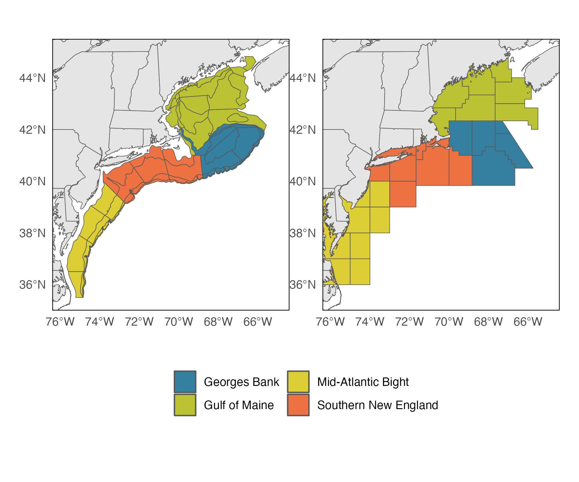{fig-align="center"}\## Ecological IndicatorsFor each region we developed the following time series of ecological indicators:1. Annual mean abundance and biomass by functional group\2. Annual mean length and weight of the aggregate community and for each functional group\3. Annual estimates of the community size spectrum slopeTotal abundance and biomass for each sub-region were calculated for each year using area-stratified abundance and the estimates of weight-at-length from Wigley et al. 2003. This process was repeated for each region and for each of the four functional groups. This gave us longitudinal changes to abundance and biomass for the aggregate community and its functional components. Changes to body size were measured using the average length and weight across all 68 species. Average size estimates were weighted by area-stratified abundance. Average body length (cm) and body weight (kg) was calculated for each region and for each functional group. The data for body size estimates was not truncated using any minimum or maximum size and reflects all available catch data for the 68 species in this study. Long-term trends were determined using linear regression. Annual size spectra were calculated for each region using the extended likelihood method (MLEbin) of @edwards2020 . This method estimates the exponent of the size spectra (b) for a bounded power law relationship between length-specific abundance and length-estimated biomass. The exponent of this relationship is analogous to slope estimates from normalized biomass spectra methods that employ a linear regression on logarithmic axes @carvalho2021 . This method has been shown to be the most accurate for estimating the exponent of size spectra when tested against alternative methods ( @white2008 ; @sprules2016 ; @edwards2017 ). Using this method, the size spectra exponent (b) was estimated for each region from 1970 to 2019. A minimum body weight of 1g was used for the lower bound and a maximum biomass of 10 kg was used as an upper bound when estimating the size spectra to account for poor survey catchability at the smallest and largest sizes. This size range retained 97.83% of all the biomass for the 68 species included in this study. Exponents of size spectra (b) were calculated using code modified from the sizeSpectra package (@edwards2017; @edwards2020) and implemented using the R statistical programming language.```{r}#| label: biomass-group-summaries# This cell provides the group summaries for how much biomass exists in each size/functional group# Actual log10 bins# Do some grouping by year survey area and functional groupfgroup_area <-log2_bin_summaries(data_in = catch_size_bins, Year, survey_area, hare_group)fgroup_all <-log2_bin_summaries(data_in = catch_size_bins, Year, hare_group)fgroup_all <- fgroup_all %>%map(function(x){mutate(x, survey_area ="Northeast Shelf")})# Join the overall values back infgroup_area <-map2(fgroup_area, fgroup_all, bind_rows)# Add new units in millionsfgroup_area$weight_bins <- fgroup_area$weight_bins %>%mutate(strat_abund_mill = wtbin_strat_abund /1e6,strat_lwbio_mill = wtbin_strat_lw_bio /1e6,survey_area =factor(survey_area,levels = area_levels))``````{r}#| label: body-size-data# Load the average body size datawithr::with_dir(rprojroot::find_root('_targets.R'), tar_load(mean_sizes_ss_groups)) # Overall across all regionsshelf_size <- mean_sizes_ss_groups %>%filter(`group ID`=="single years") %>%mutate(survey_area ="Northeast Shelf")# Grouped on year and regionregional_size <- mean_sizes_ss_groups %>%filter(`group ID`=="single years * region") %>%bind_rows(shelf_size) %>%mutate(Year =as.numeric(Year),survey_area =as.character(survey_area)) %>%left_join(area_df) %>%mutate(area_titles =factor(area_titles, levels = area_levels_long),area_copy = survey_area)# 2. Grouped on year, region, & functional groupfunctional_group_size <- mean_sizes_ss_groups %>%filter(`group ID`=="single years * region * functional group") %>%mutate(Year =as.numeric(Year),survey_area =factor(survey_area, levels = area_levels))# Refactor areasfunctional_group_size <- functional_group_size %>%mutate(survey_area =as.character(survey_area)) %>%left_join(area_df) %>%mutate(area_titles =factor(area_titles, levels = area_levels_long),area_copy = survey_area)``````{r}#| label: plotting-bigfish-smallfish#| eval: false# Idea: it would be great top be able to speak more directly to population trends for large/small individuals within a functional group...# One avenue is to break it into large/small# Could use the median body sizesize_trends <- catch_size_bins %>%mutate(fish_size =ifelse(wmin_g >1000, "Over 1kg", "Less than 1 kg")) %>%group_by(Year,area, hare_group, fish_size) %>%summarise(total_abund =sum(strat_total_abund_s)/1e6,total_biomass =sum(strat_total_lwbio_s), .groups ="drop") %>%pivot_longer(cols =c(total_abund, total_biomass), names_to ="var", values_to ="vals") # Abundancesize_trends %>%filter(var =="total_abund") %>%#filter(var == "total_biomass") %>% filter(hare_group %in%c("groundfish", "elasmobranch")) %>%ggplot(aes(Year, vals)) +geom_point(aes(color = fish_size), size =0.5) +geom_smooth(aes(color = fish_size), linewidth =1, se = F) +scale_color_gmri() +scale_y_continuous(labels = scales::comma_format()) +facet_grid(area~hare_group) +labs(color ="Fish Size", y ="Abundance (millions)" )# Biomasssize_trends %>%#filter(var == "total_abund") %>% filter(var =="total_biomass") %>%filter(hare_group %in%c("groundfish", "elasmobranch")) %>%ggplot(aes(Year, vals)) +geom_point(aes(color = fish_size), size =0.5) +geom_smooth(aes(color = fish_size), linewidth =1, se = F) +scale_color_gmri() +scale_y_continuous(labels = scales::comma_format()) +facet_grid(area~hare_group) +labs(color ="Fish Size", y ="Biomass (kg)" )``````{r}#| label: load the size spectrum indiceswithr::with_dir(rprojroot::find_root('_targets.R'), tar_load(size_spectrum_indices)) # Grab the overall shelf-wide SSshelf_ss <- size_spectrum_indices %>%filter(`group ID`=="single years") %>%mutate(survey_area ="Northeast Shelf")# Grab SS Groups for each regionregion_indices <- size_spectrum_indices %>%filter(`group ID`=="single years * region") %>%bind_rows(shelf_ss) %>%mutate(yr =as.numeric(as.character(Year)),survey_area =factor(survey_area, levels = area_levels),sig_fit =ifelse(log2_sig_strat <0.05, "Significant", "Non-Significant"))# Make a copy so we can gray out the lines in plots# Merge the long names for labels "area_titles"region_indices <- region_indices %>%mutate(survey_area =as.character(survey_area)) %>%left_join(area_df) %>%mutate(area_titles =factor(area_titles, levels = area_levels_long),area_copy = survey_area)```## Drivers of Spectra ChangeImpacts of external factors on spectra slope were explored using multiple regression analyses. Annual variation in regional slope was modeled using measures of large-scale environmental conditions, anthropogenic disturbance, and bottom up resource quality. Environmental drivers were the regional SST anomalies and the Gulf Stream Index (GSI). Global SST data were obtained via NOAA's Optimum Interpolation SST analysis (OISSTv2), which provides daily SST values at a 0.25° latitude x 0.25° longitude resolution @reynolds2007 . A daily climatology for every 0.25° pixel in the global data set was created using average daily temperatures spanning the period of 1982-2011. Daily anomalies were then computed as the difference between observed temperatures and the daily climatological average. OISSTv2 data used in these analyses were obtained from the NOAA Physical Sciences Laboratory, Boulder, Colorado, USA from their website. SST anomalies were regionally averaged to produce time series for each of the four survey sub-regions described above (Figure 1a). These were then averaged to within years to form annual time series of SST anomalies. The Gulf Stream index (GSI) quantifies the latitude of the Gulf Stream position based on ocean temperatures at 200 m depth between 55° W and 75° W longitude. The index was obtained from the ecodata package in R (Bastille & Hardison 2018), which supplies GSI data at monthly intervals following the methodology of Pérez-Hernández and Joyce (2014) and @joyce2019 , using sea level height anomaly data from the Copernicus Marine Environment Monitoring Service. Fishing pressure represents the primary top-down anthropogenic driver in the region, and was investigated using regional commercial landings data. Fishing pressure in the region was measured using state and federal commercial fishing landings. This data was obtained from the Greater Atlantic Regional Fisheries Office (GARFO) for statistical areas that are routinely used for fisheries reporting and management. Individual statistical areas were aggregated into clusters that closely aligned with the trawl survey areas (Figure 1b). Bottom-up ecological interactions were explored using two zooplankton indices. Zooplankton indices were from NOAA Fisheries' Marine Resources Monitoring, Assessment and Prediction (MARMAP) program and Ecosystem Monitoring (EcoMon) cruises ( @morse2017 ). Abundance anomalies were computed from the expected abundance on the day of sample collection. The small copepod index is computed by averaging the individual abundance anomalies of Pseudocalanus spp., Centropages hamatus, Centropages typicus, and Temora longicornis. The "large-copepod" anomaly values are the abundance anomaly of Calanus finmarchicus, the largest copepod in the Northeast U.S. region ( @kane2007 , @kane2008 ). Anomalies for both large and small zooplankton groups were averaged within ecological production units by the data provider, producing annual timeseries for the Gulf of Maine, Georges Bank, and Mid-Atlantic Bight (NMFS 2023). The zooplankton timeseries for the Mid-Atlantic Bight EPU was used for both the Mid-Atlantic Bight and Southern New England regions in our analyses due to shared geographic overlap. Each of these drivers (climate, primary productivity, fishing) have independently been shown in other works to have measurable impacts on size spectra ( @duplisea1995 ; @blanchard2005 ; @woodworth-jefcoats2020 ). Our exploratory investigations here are an effort to evaluate which predictors most explain the variance seen in the regional size spectra, and whether those relationships have changed over the study period. To highlight potential cases of non-stationarity, a hallmark of regime-shift dynamics ( @blöcker2023) , we explored the temporal structures in the regional spectra using breakpoint analyses. Breakpoint analyses were performed using the envcpt package (Killick et al. 2021). This package applies an automatic model selection process testing support for candidate model structures including constant/piecewise changes to the mean, variance, trends, & autocorrelations and any identified changepoints located using the pruned exact linear time algorithm ( @rikardsen2004 ). Results from the breakpoint analysis were used to identify whether regional spectra expressed distinct periods of change. In cases where changepoints were identified an additional "regime" term was included to the regression analyses of key drivers. This term allowed for non-linear driver effects across different periods of time. Time-lags on predictors were also evaluated to explore important non-contemporaneous relationships between drivers and size spectra. Important lagged relationships were identified through the use of cross correlation function (CCF) estimates. CCFs were performed for the dependent variable of the size spectra slope with the independent variables of SST, GSI, commercial fisheries landings, and small and large zooplankton indices for annual lags up to 10 years. Significant lags were then included as additional candidate predictors in the multiple regression analysis of spectrum slope changes. Multiple regression models were evaluated independently for each region and their performances using AICc to rank the most parsimonious models.```{r}#| label: gsi-data-prep#| eval: true#### 2. Climate Drivers ##### From ecodata: GSI & Zooplankton#### GSI# Gulf Stream Indexgsi <- ecodata::gsi %>%mutate(Time =str_pad(as.character(Time), width =7, side ="right", pad ="0"),year =as.numeric(str_sub(Time, 1, 4)),month =str_sub(Time, -2, -1),Time =as.Date(str_c(year, month, "01", sep ="-")))``````{r}#| label: load temperature data# Load the regional temperatures from {targets}withr::with_dir(rprojroot::find_root('_targets.R'), tar_load(regional_oisst))# Get regional averagestemp_regimes <- regional_oisst %>%filter(yr >1981) %>%mutate(regime =ifelse(sst_anom >0, "hot", "cold"),survey_area =ifelse( survey_area =="all", "Northeast Shelf", survey_area),survey_area =factor(survey_area, levels = area_levels)) ``````{r}#| label: garfo-data-prep#| eval: true#### GARFO Landings ##### Load the GARFO landings data:# Landings of finfish* sheet 5landings <-read_xlsx(path =str_c(res_path, "GARFO_landings/KMills_landings by area 1964-2021_JUN 2022.xlsx"), sheet =5) %>%rename_all(tolower)# Add the labels into the landings data and remove what we don't need there:landings <- landings %>%mutate(survey_area =case_when(`stat area`%in% fish_zones$"Gulf of Maine"~"Gulf of Maine",`stat area`%in% fish_zones$"Georges Bank"~"Georges Bank",`stat area`%in% fish_zones$"Southern New England"~"Southern New England",`stat area`%in% fish_zones$"Mid-Atlantic Bight"~"Mid-Atlantic Bight")) %>%filter(survey_area %in%c("Georges Bank", "Gulf of Maine", "Southern New England", "Mid-Atlantic Bight")) %>%mutate(survey_area =factor(survey_area, area_levels_long))# Get Summarieslandings_summ <- landings %>%drop_na() %>%rename("weight_lb"=`landed lbs`,"live_lb"=`live lbs`) %>%drop_na() %>%group_by(year, survey_area) %>%summarise( across(.cols =c(value, weight_lb, live_lb), .fns =list(mean =~mean(.x , na.rm = T), total =~sum(.x , na.rm = T)), .names ="{.fn}_{.col}"), .groups ="drop") # Scale the landings to create an index by arealandings_summ <- landings_summ %>%group_by(survey_area) %>%mutate(total_wt_z =as.numeric(base::scale(total_weight_lb))) %>%ungroup()``````{r}#| label: zp-data-prep# ADD Zooplankton: small and large zooplankton anomalies for the EPUS# Don't need to scale# Load original datazp_sli <- ecodata::zoo_sli_anom %>%filter(EPU !="SS")# Reformat to match the other indiceszp_index <- zp_sli %>%#EPUS combine SNE and MAB, we can repeat the values herebind_rows(filter(zp_sli, EPU =="MAB") %>%mutate(EPU ="SNE")) %>%mutate(survey_area =case_when( EPU =="GB"~"Georges Bank", EPU =="GOM"~"Gulf of Maine", EPU =="MAB"~"Mid-Atlantic Bight", EPU =="SNE"~"Southern New England"),Units =str_c("zp_", Var)) %>%select(year = Time, survey_area, Value, Units) %>%pivot_wider(names_from = Units, values_from = Value)``````{r}#| label: combine-drivers-table#### Build a Common form for all Drivers: ##### Format: year, area, var, value#---#### Reshape all the inputs so that we can bind them together in one dataframe# 1.Climate Features# Join the climate modes togetherclim_drivers <- gsi %>%filter(EPU =="All")# Put climate drivers on annual scheduleclim_idx <- clim_drivers %>%group_by(year, area = EPU, var = Var) %>%summarise(value =mean(Value, na.rm = T),.groups ="drop")#---# 2. GARFO landingslandings_idx <- landings_summ %>%group_by(year, area = survey_area) %>%summarise(value =mean(total_wt_z, na.rm = T),.groups ="drop") %>%mutate(var ="landings")#---# 3. Temperaturesst_idx <- temp_regimes %>%left_join(area_df, by ="survey_area") %>%select(year = yr, area, value = sst_anom) %>%mutate(var ="sst_anom")#---# 4. Zooplanktonzp_idx <- zp_index %>%pivot_longer(cols =c(zp_small, zp_large), names_to ="var", values_to ="value") %>%rename(area = survey_area)#---# 4. Size Spectrum Slopes & Interceptsss_idx <- region_indices %>%select(year = Year, survey_area, spectra_slope = log2_slope_strat, #spectra_int = log2_int_strat,isd_slope = b) %>%pivot_longer(# cols = c(spectra_slope, spectra_int, isd_slope), cols =c(spectra_slope, isd_slope), names_to ="var", values_to ="value") %>%mutate(year =as.numeric(year)) %>%left_join(area_df, by ="survey_area") %>%select(-survey_area)#---# All Metrics Togetherall_drivers <-bind_rows(list( clim_idx, landings_idx, sst_idx, zp_idx, ss_idx))``````{r}#| label: driver-scaling# In this chunk the drivers get reshaped to scale# Scaling should cover the period of analysis 1982-2019# SST and GSI (all index/anomaly fields) are not scaled# Put the data in a wide form for scaling:drivers_wide <- all_drivers %>%filter(year >=1982, year <=2019) %>%mutate(id =str_replace_all(str_c(area, "_", var), " ", "_")) %>%select(-c(area, area_titles, var)) %>%pivot_wider(names_from = id, values_from = value) %>%column_to_rownames(var ="year")# Scale the landings, not SST or GSIto_scale <-select(drivers_wide, ends_with("landings")) %>%scale() %>%as.data.frame()dont_scale <-select(drivers_wide, -ends_with("landings"))# Join back togetherdrivers_scaled <-bind_cols(dont_scale, to_scale) %>%rownames_to_column(var ="year")``````{r}#| label: driver-correlation-periods# Pull different years into a listdriver_periods <-list("1982-1998"=c(1982:1998),"1999-2006"=c(1999:2006),"2007-2019"=c(2007:2019),"1982-2019"=c(1982:2019))# -------------------------------------------------# Idea: Add functional_group_sizes into the correlation chart:# Reshape the size information so we can combine it with the drivers:# Values are scaled heresizes_wide <- functional_group_size %>%select(year = Year, survey_area, hare_group, avg_weight = mean_wt_kg) %>%pivot_longer(names_to ="var", values_to ="value", cols =c(avg_weight)) %>%inner_join(area_df, by ="survey_area") %>%select(-survey_area) %>%mutate(id =str_replace_all(str_c(area, "_", hare_group, "_", var), " ", "_")) %>%select(-c(area, area_titles, var, hare_group)) %>%pivot_wider(names_from = id, values_from = value, values_fn = {mean}) %>%column_to_rownames(var ="year") %>%scale() %>%as.data.frame()# Join regional size changes to the scaled driversdrivers_and_sizes <- drivers_scaled %>%left_join(rownames_to_column(sizes_wide, var ="year"), by ="year") %>%column_to_rownames(var ="year")# Split them out into a list that contains data for each period# Takes the years in driver_periods and pulls the rows that corresponddriver_period_list <-map(driver_periods, function(yrs){ period_matrix <- drivers_and_sizes[rownames(drivers_and_sizes) %in% yrs, ] %>%drop_na()})``````{r}#| label: regression-analysis-data# Use scaled drivers for the regressions# Need to drop zooplankton because they are non-unique since we split the MAB EPU and repeated itregression_df <- drivers_scaled %>%select(!ends_with(c("zp_small","zp_large")))# Build back out the metadata:# Identify what region is associated with both: spectrum values & driver valuesregression_df <- regression_df %>%pivot_longer(names_to ="spectra_param", values_to ="spectra_values", cols =ends_with("slope") |ends_with("int")) %>%pivot_longer(names_to ="driver_var", values_to ="driver_values", cols =-matches("spectra|year")) %>%mutate(year =as.numeric(year),# A. Flag what the driver type wasdriver_type =case_when(str_detect(driver_var, "landings") ~"Commercial Landings",str_detect(driver_var, "sst") ~"SST",str_detect(driver_var, "index") ~"GSI",TRUE~"Missed Something"),# B. Flag what the spectrum feature wasparam_feature =case_when(# Flag what the Size Distribution Parameter wasstr_detect(spectra_param, "int") ~"Spectra Intercept",str_detect(spectra_param, "isd") ~"ISD Exponent",str_detect(spectra_param, "slope") ~"Spectra Slope",TRUE~"Missed Something"),# C. These are the areas associated with the Spectra Featuresspectra_area =case_when(str_detect(spectra_param, "All") ~"All",str_detect(spectra_param, "Georges") ~"Georges Bank",str_detect(spectra_param, "Gulf") ~"Gulf of Maine",str_detect(spectra_param, "Southern") ~"Southern New England",str_detect(spectra_param, "Mid-Atlantic") ~"Mid-Atlantic Bight"),spectra_area =factor(spectra_area, levels =c("All", "Gulf of Maine", "Georges Bank", "Southern New England", "Mid-Atlantic Bight")),# D. These are the areas of the driversdriver_area =case_when(str_detect(driver_var, "All") ~"All",str_detect(driver_var, "Georges") ~"Georges Bank",str_detect(driver_var, "Gulf") ~"Gulf of Maine",str_detect(driver_var, "Southern") ~"Southern New England",str_detect(driver_var, "Mid-Atlantic") ~"Mid-Atlantic Bight"),driver_area =factor(driver_area, levels =c("All", "Gulf of Maine", "Georges Bank", "Southern New England", "Mid-Atlantic Bight")),# E. Add Decade indecade =floor_decade(year),##regime = ifelse(year < 2010, "regime_1", "regime_2" ) ) # Filter it so predictors are only within matching regions, # or just overarching (GSI)regression_df <- regression_df %>%filter(driver_area == spectra_area | driver_type =="GSI") %>%arrange(year, driver_var)# Last wrangling:# columns for: year, slope, isd, spectra region, drver_region, GSI, sst_anom, landings# GSI is so annoying here, just rejoin it without the area columnregression_df <- regression_df %>%select(-c(spectra_param, driver_var)) %>%pivot_wider(names_from ="driver_type", values_from ="driver_values") %>%pivot_wider(names_from ="param_feature", values_from ="spectra_values") %>%select(-GSI) %>%filter(driver_area !="All") %>%left_join( select(clim_idx, year, GSI = value), by =c("year") ) %>%mutate(spectra_area =fct_drop(spectra_area))# Add zooplankton here so it can be checked in the regressions# Zooplankton values are duplicated in MAB and SNE b/c its the same EPUregression_df <-left_join( regression_df, zp_index %>%rename(spectra_area = survey_area), by =join_by(year, spectra_area))```# Results## Abundance and Biomass ChangesAbundance has been gradually increasing on the Northeast Shelf since 1970, accelerating after 2007 to peak levels in 2014. Following that peak, shelf-wide numbers have been in decline (Figure 2). In the Gulf of Maine, fish abundance was relatively low until the 1990's when it began to steadily rise. Abundance here fell during 2002-2006, but then continued to rise after 2006. Gulf of Maine abundance peaked in 2016 and then declined through 2019. Georges Bank abundance was low from 1970 through 2010. By 2014 abundance had roughly quadrupled, propelled by notable strong recruitment classes of haddock and other groundfish species. After peaking in 2014, abundance soon fell to levels more similar to the 1970-2010. Abundance in Southern New England displayed higher inter-annual variability when compared to both Gulf of Maine and Georges Bank. Abundance began increasing rapidly in 2007, before falling back to earlier levels by the end of the 2010's. The Mid Atlantic Bight displayed a similar inter-annual variability, but had no major trend in fish abundance. Groundfish species were the dominant functional group driving the abundance and trends in the Gulf of Maine and Georges Bank, contributing more than half the total fish abundance in these regions. The two southern regions showed a more balanced abundance distribution among the five functional groups, with a larger representation of coastal and diadromous species (Figure 2). Shelf-wide biomass has been on the rise since the late-1990's. Biomass peaked in 2016, and fell for the next three years mirroring the pattern seen in abundance (Figure 2). Shelf biomass was concentrated among two major functional groups, groundfish and elasmobranchs. Groundfish biomass was lowest in the late 80's and early 90's, before rebounding in the 2000's. Elasmobranch biomass increased throughout the study period, with the exception of southern New England (Figure 2). Biomass was higher in the two northern regions, the Gulf of Maine and Georges Bank. The Gulf of Maine followed a similar trend to the shelf as a whole. Biomass here was at its lowest during the 1980's, but had more than doubled by 2000 and in years following, peaking in 2016 before declining each year after. The majority of the biomass here was found among groundfish and elasmobranch species. Georges Bank had a similar groundfish and elasmobranch composition. Biomass here was lowest in the early 1970's. During the 1980's groundfish biomass declined, but this was offset by growth in elasmobranch species. The region hit low biomass levels again in the 1990's before climbing to peak levels in 2014. Biomass then fell here each year after. .In Southern New England the biomass changes were less steady. Increases in the 1980's were followed by abrupt declines in the mid 1990's. The region saw its highest biomass in 2012, with a familiar decline towards the end of the timeseries. Biomass here was represented with a majority role of elasmobranch species. This was also the case in the Mid-Atlantic Bight, a region that saw long term growth in its biomass and a peak in 2019.```{r}#| label: abundance and biomass summary numbers#---- Overall Abundance Trends# Total abundance and biomass for the whole shelfshelf_summary <- catch_size_bins %>%group_by(Year) %>%summarise(lwbio_mill =sum(strat_total_lwbio_s, na.rm = T) /1e6,abund_mill =sum(strat_total_abund_s, na.rm = T) /1e6)# Total Abundance and Biomass for the regionsregion_summary <- catch_size_bins %>%left_join(area_df) %>%group_by(Year, area_titles) %>%summarise(lwbio_mill =sum(strat_total_lwbio_s, na.rm = T) /1e6,abund_mill =sum(strat_total_abund_s, na.rm = T) /1e6,.groups ="drop") %>%mutate(area_titles =factor(area_titles, levels = area_levels_long))# Total abundance and biomass for functional Groups within the regionsfunctional_group_summary <- catch_size_bins %>%left_join(area_df) %>%group_by(Year, area_titles, hare_group) %>%summarise(lwbio_mill =sum(strat_total_lwbio_s, na.rm = T) /1e6,abund_mill =sum(strat_total_abund_s, na.rm = T) /1e6,.groups ="drop") %>%mutate(area_titles =factor(area_titles, levels = area_levels_long))``````{r}#| label: abundance totals by area#| eval: true#| fig.width: 8#| fig-height: 6# Abundance 1.shelf_abund_p <- shelf_summary %>%mutate(area_titles ="Northeast Shelf") %>%ggplot() +geom_line(aes(Year, abund_mill), color =gmri_cols("dark gray"), linewidth =1) +#geom_col(aes(Year, abund_mill), fill = gmri_cols("dark gray")) +scale_y_continuous(labels =label_comma()) +facet_wrap(~area_titles) +labs(y ="Abundance (millions)")# Abundance 2.region_abund_p <- region_summary %>%ggplot() +geom_col(aes(Year, abund_mill, fill = area_titles), show.legend = F, width =1) +scale_fill_gmri() +scale_y_continuous(labels =label_comma()) +facet_wrap(~area_titles, ncol =1, scales ="free") +labs(y ="Abundance (millions)")abund_trendz <- shelf_abund_p | region_abund_pabund_trendz```#### Regional Abundances::: panel-tabset##### Northeast Shelf```{r}#| fig.width: 8#| fig-height: 6shelf_fgroup_summary <- catch_size_bins %>%mutate(area_titles ="Northeast Shelf") %>%group_by(Year, area_titles, hare_group) %>%summarise(lwbio_mill =sum(strat_total_lwbio_s, na.rm = T) /1e6,abund_mill =sum(strat_total_abund_s, na.rm = T) /1e6,.groups ="drop")# Make Plot for Functional Groupsshelf_fgroup_abund_p <- shelf_fgroup_summary %>%ggplot() +geom_col(aes(Year, abund_mill, fill = hare_group), show.legend = F) +scale_fill_gmri() +scale_y_continuous(labels =label_comma()) +facet_wrap(~hare_group, ncol =1, scales ="free") +labs(y ="Abundance (millions)")# Place Functional Groups Beside Shelfshelf_abund_p | shelf_fgroup_abund_p```##### Gulf of Maine```{r}#| fig.width: 8#| fig-height: 6area_option <-"Gulf of Maine"plot_area_abund_summary <-function(area_option){ area_abund_p <- region_summary %>%filter(area_titles == area_option) %>%ggplot() +geom_line(aes(Year, abund_mill), color =gmri_cols("dark gray"), linewidth =1) +#geom_col(aes(Year, abund_mill), fill = gmri_cols("dark gray")) +scale_y_continuous(labels =label_comma()) +facet_wrap(~area_titles) +labs(y ="Abundance (millions)")# Make Plot for Functional Groupsarea_fgroup_abund_p <- functional_group_summary %>%filter(area_titles == area_option) %>%ggplot() +geom_col(aes(Year, abund_mill, fill = hare_group), show.legend = F) +scale_fill_gmri() +scale_y_continuous(labels =label_comma()) +facet_wrap(~hare_group, ncol =1, scales ="free") +labs(y ="Abundance (millions)")# Place Functional Groups Beside Shelfp_out <- area_abund_p | area_fgroup_abund_preturn(p_out)}plot_area_abund_summary(area_option ="Gulf of Maine")```##### Georges Bank```{r}#| fig.width: 8#| fig-height: 6plot_area_abund_summary(area_option ="Georges Bank")```##### Southern New England```{r}#| fig.width: 8#| fig-height: 6plot_area_abund_summary(area_option ="Southern New England")```##### Mid-Atlantic Bight```{r}#| fig.width: 8#| fig-height: 6plot_area_abund_summary(area_option ="Mid-Atlantic Bight")```:::### Biomass Changes```{r}#| label: biomass totals by area#| fig.width: 8#| fig-height: 6#----- Overall Biomass# Repeat for Biomass# Abundance 1.shelf_bio_p <- shelf_summary %>%mutate(area_titles ="Northeast Shelf") %>%ggplot() +geom_line(aes(Year, lwbio_mill), color =gmri_cols("dark gray"), linewidth =1) +#geom_col(aes(Year, abund_mill), fill = gmri_cols("dark gray")) +scale_y_continuous(labels =label_comma()) +facet_wrap(~area_titles) +labs(y ="Biomass (million kg)")# Abundance 2.region_bio_p <- region_summary %>%ggplot() +geom_col(aes(Year, lwbio_mill, fill = area_titles), show.legend = F, width =1) +scale_fill_gmri() +scale_y_continuous(labels =label_comma()) +facet_wrap(~area_titles, ncol =1, scales ="free") +labs(y ="Biomass (million kg)")biomass_trendz <- shelf_bio_p | region_bio_pbiomass_trendz```#### Regional Biomass::: panel-tabset##### Northeast Shelf```{r}#| fig.width: 8#| fig-height: 6#| label: ne-shelf-biomass# Make Plot for Functional Groupsshelf_fgroup_bio_p <- shelf_fgroup_summary %>%ggplot() +geom_col(aes(Year, lwbio_mill, fill = hare_group), show.legend = F) +scale_fill_gmri() +scale_y_continuous(labels =label_comma()) +facet_wrap(~hare_group, ncol =1, scales ="free") +labs(y ="Biomass (million kg)")# Place Functional Groups Beside Shelfshelf_bio_p | shelf_fgroup_bio_p```##### Gulf of Maine```{r}#| fig.width: 8#| fig-height: 6#| label: gom-biomassarea_option <-"Gulf of Maine"plot_area_bio_summary <-function(area_option){ area_bio_p <- region_summary %>%filter(area_titles == area_option) %>%ggplot() +geom_line(aes(Year, lwbio_mill), color =gmri_cols("dark gray"), linewidth =1) +scale_y_continuous(labels =label_comma()) +facet_wrap(~area_titles) +labs(y ="Biomass (million kg)")# Make Plot for Functional Groupsarea_fgroup_bio_p <- functional_group_summary %>%filter(area_titles == area_option) %>%ggplot() +geom_col(aes(Year, lwbio_mill, fill = hare_group), show.legend = F) +scale_fill_gmri() +scale_y_continuous(labels =label_comma()) +facet_wrap(~hare_group, ncol =1, scales ="free") +labs(y ="Biomass (million kg)")# Place Functional Groups Beside Shelfp_out <- area_bio_p | area_fgroup_bio_preturn(p_out)}plot_area_bio_summary(area_option ="Gulf of Maine")```##### Georges Bank```{r}#| fig.width: 8#| fig-height: 6#| #| label: gb-biomassplot_area_bio_summary(area_option ="Georges Bank")```##### Southern New England```{r}#| fig.width: 8#| fig-height: 6#| #| label: sne-biomassplot_area_bio_summary(area_option ="Southern New England")```##### Mid-Atlantic Bight```{r}#| fig.width: 8#| fig-height: 6#| #| label: mab-biomassplot_area_bio_summary(area_option ="Mid-Atlantic Bight")```:::### Body-Size ChangesNortheast shelf length and weight of the "average" individual fish has remained relatively stable over nearly five decades (Figure 2.). Average length did not change over the study, averaging 26.06 cm (sd = 2.57). Average weight declined slowly at 8.95g year-1 of the same period.Independent trends were found within the regional communities. Fish size declines in the Gulf of Maine were the most of any region. Average length was highest in the 1970s & 1980s at around 34.7-34.8 cm, lengths fell to 28 cm in the last decade with an overall trend of -.19 cm year-1 . The average weight also fell during the 1980s, from an average of 0.8 kg in the 1970s to 0.3 kg in the 2010s, a decline of 62.5% and a long-term rate of -1.1g year-1 . Georges Bank average sizes declined in average weight (-5.48g year-1), but with no overall change in length. Declining sizes for both the Gulf of Maine and Georges Bank slowed during the late 2000s, but then continued to fall the following decade. Average body size in southern New England was relatively constant, with no long-term changes in length or weight. The Mid-Atlantic Bight region was the only area with long-term increases in both length (.26cm year-1) and weight (4.89g year-1) during the study period.::: panel-tabset#### All Species```{r}#| label: regional-size-trends#| fig.height: 8# Re-factorregional_size <- regional_size %>%filter(Year <2020) %>%mutate(survey_area =factor(survey_area, area_levels),area_copy = survey_area)# Get the average length and weight at each decadeavg_size_decades <- regional_size %>%mutate(decade_left =as.numeric(as.character(floor_decade(Year))),decade_right =as.numeric(as.character(floor_decade(Year+10))) -1,decade_center = (decade_left + decade_right)/2,decade_lab =str_c(decade_left, "-", decade_right)) %>%group_by(area_titles, decade_left, decade_right, decade_center, decade_lab) %>%summarise(mean_len_cm =mean(mean_len_cm),mean_wt_kg =mean(mean_wt_kg),.groups ="drop" )# Length plotavg_len_p <- regional_size %>%ggplot() +geom_line(aes(Year, mean_len_cm, group = area_titles), linewidth =1,show.legend = F, color ="gray60") +geom_segment(data = avg_size_decades,aes(x = decade_left, xend = decade_right, y = mean_len_cm, yend = mean_len_cm), linewidth =1.5) +geom_text(data = avg_size_decades,aes(x = decade_center, y = mean_len_cm, label =str_c(round(mean_len_cm, 1)) ), vjust =-2.25, size =4, fontface ="bold") +scale_color_gmri() +facet_wrap(~area_titles, ncol =1, scales ="free") +scale_y_continuous(expand =expansion(mult =c(0.1, 0.55))) +labs(title ="Average Length",y ="Length (cm)",color ="Region")# Weight plotavg_wt_p <- regional_size %>%ggplot(aes(Year, mean_wt_kg)) +geom_line(aes(group = area_titles), linewidth =1,show.legend = F,color ="gray60") +geom_segment(data = avg_size_decades,aes(x = decade_left, xend = decade_right, y = mean_wt_kg, yend = mean_wt_kg), linewidth =1.5) +geom_text(data = avg_size_decades,aes(x = decade_center, y = mean_wt_kg, label =str_c(round(mean_wt_kg, 2)) ), vjust =-2.25, size =4, fontface ="bold") +scale_color_gmri() +scale_y_continuous(expand =expansion(mult =c(0.1, 0.55))) +facet_wrap(~area_titles, ncol =1, scales ="free") +labs(title ="Average Weight",y ="Weight (kg)",color ="Region")# Plot side by side(avg_len_p | avg_wt_p) ```#### Functional Group Avg. Length```{r}#| label: functional-group-length-trends#| fig-height: 6# Get the average length and weight at each decadeavg_fgroup_decades <- functional_group_size %>%mutate(decade_left =as.numeric(as.character(floor_decade(Year))),decade_right =as.numeric(as.character(floor_decade(Year+10))) -1,decade_center = (decade_left + decade_right)/2,decade_lab =str_c(decade_left, "-", decade_right)) %>%group_by(area_titles, hare_group, decade_left, decade_right, decade_center, decade_lab) %>%summarise(mean_len_cm =mean(mean_len_cm),mean_wt_kg =mean(mean_wt_kg),.groups ="drop")# Plot the Length changesfunctional_group_size %>%ggplot() +geom_line(aes(Year, mean_len_cm, group = area_titles), linewidth =1,show.legend = F, color ="gray60") +geom_segment(data = avg_fgroup_decades,aes(x = decade_left, xend = decade_right, y = mean_len_cm, yend = mean_len_cm), linewidth =1.5) +geom_text(data = avg_fgroup_decades,aes(x = decade_center, y = mean_len_cm, #y = Inf,label =str_c(round(mean_len_cm, 1)) ), vjust =-2.5, #vjust = 1.75,size =3.5, fontface ="bold") +scale_y_continuous(expand =expansion(mult =c(0.1, 0.4))) +scale_color_gmri() +facet_grid(hare_group~area_titles, scales ="free_y") +labs(title ="Average Length",y ="Length (cm)",color ="Region")```#### Functional Group Avg. Weight```{r}#| label: functional-group-weight-trends#| fig-height: 6# Average Weightsfunctional_group_size %>%ggplot() +geom_line(aes(Year, mean_wt_kg, group = area_titles), linewidth =1,show.legend = F, color ="gray60") +geom_segment(data = avg_fgroup_decades,aes(x = decade_left, xend = decade_right, y = mean_wt_kg, yend = mean_wt_kg), linewidth =1.5) +geom_text(data = avg_fgroup_decades,aes(x = decade_center, y = mean_wt_kg, label =str_c(round(mean_wt_kg, 1)) ), vjust =-2.5, size =3.5, fontface ="bold") +scale_y_continuous(expand =expansion(mult =c(0.1, 0.4))) +scale_color_gmri() +facet_grid(hare_group~area_titles, scales ="free_y") +labs(title ="Average Weight",y ="Weight (kg)",color ="Region")```:::##### Population and Size Changes Combined```{r}#| label: assembline-overall-and-regional-size-changes# Mirror the abundance and biomass layouts, they look good# Length 1.shelf_len_p <- regional_size %>%filter(area_titles =="Northeast Shelf") %>%ggplot() +geom_line(aes(Year, mean_len_cm), color =gmri_cols("dark gray"), linewidth =1) +scale_y_continuous(labels =label_comma()) +facet_wrap(~area_titles) +labs(y ="Average Length (cm)")# Length 2.region_len_p <- regional_size %>%filter(area_titles !="Northeast Shelf") %>%mutate(Year =as.numeric(Year)) %>%ggplot() +geom_col(aes(Year, mean_len_cm, fill = area_titles), show.legend = F, width =1) +scale_fill_gmri() +scale_y_continuous(labels =label_comma()) +facet_wrap(~area_titles, ncol =1, scales ="free") +labs(y ="Average Length (cm)")# Assemblelen_trendz <- shelf_len_p | region_len_p# Weight 1.shelf_wt_p <- regional_size %>%filter(area_titles =="Northeast Shelf") %>%ggplot() +geom_line(aes(Year, mean_wt_kg), color =gmri_cols("dark gray"), linewidth =1) +scale_y_continuous(labels =label_comma()) +facet_wrap(~area_titles) +labs(y ="Average Weight (kg)")# Weight 2.region_wt_p <- regional_size %>%filter(area_titles !="Northeast Shelf") %>%ggplot() +geom_col(aes(Year, mean_wt_kg, fill = area_titles), show.legend = F, width =1) +scale_fill_gmri() +scale_y_continuous(labels =label_comma()) +facet_wrap(~area_titles, ncol =1, scales ="free") +labs(y ="Average Weight (kg)")# Assemblewt_trendz <- shelf_wt_p | region_wt_p``````{r}#| label: pop-and-size-quad#| fig-height: 8#| fig-width: 8# Assemble the 4 panels# Row 1: population trendspop_trendz <- abund_trendz[[1]] | abund_trendz[[2]] +labs(y =NULL) | biomass_trendz[[1]] | biomass_trendz[[2]] +labs(y =NULL)pop_trendz <- pop_trendz &theme(plot.margin =margin(5,5,5,5))# Row 2: Size Trendssize_trendz <- len_trendz[[1]] | len_trendz[[2]] +labs(y =NULL) | wt_trendz[[1]] | wt_trendz[[2]] +labs(y =NULL)size_trendz <- size_trendz &theme(plot.margin =margin(5,5,5,5))# All of thempop_trendz / size_trendz```::: panel-tabset##### Size Class Dominance```{r}#| label: dom-species-plot-fun# Plotting Functionplot_dom_species <-function(bin_metrics, reg_choice, title =NULL, subtitle =NULL, add_rect =FALSE){# Plot the functional groupsdom_data <- bin_metrics %>%group_by(area_titles, bin_label, Year, metric) %>%summarise( all_total =sum(totals), .groups ="drop") %>%right_join(bin_metrics) %>%#group_by(hare_group, Year, area_titles, metric) %>% mutate(total_frac = totals / all_total) %>%ungroup() %>%filter( metric =="tot_bio", area_titles == reg_choice, hare_group %in%c("groundfish", "elasmobranch")) if(add_rect){p <-ggplot() +geom_rect(data = period_box_df, aes(xmin = xmin, xmax = xmax, ymin = ymin, ymax = ymax, fill = period), show.legend = F, alpha =0.3)}if(add_rect ==FALSE){p <-ggplot()}p <- p +geom_line(data = dom_data,aes(Year, total_frac, color = hare_group), linewidth =1) +scale_fill_gmri() +scale_color_manual(values =c("black", "#00736D")) +scale_x_continuous(limits =c(1970, 2019), expand =expansion(add =c(0.5, 0.5))) +facet_grid(bin_label~area_titles) +theme(strip.text.y =element_blank()) +scale_y_continuous(labels =percent_format()) +labs(x ="Year", y ="Percent of Total Biomass", color ="Functional Group",title = title,subtitle = subtitle) +#,#subtitle = "Functional Group Dominance") +theme(plot.margin =margin(r =0, l =1))p}``````{r}#| label: plot-sizeclass-bio-and-fraction-bio#| fig-width: 8#| fig-height: 8#--------- Plots# Set the Region:reg_choice <-"Gulf of Maine"# Okay for real:# Label size bins, do a trend line or just do a heatmap. # Heatmap will have some issues with scaling# Box to backdrop the periodsperiod_box_df <-data.frame(period =c("1972-1998", "1999-2006", "2007-2019"),xmin =c(1970, 1998.5, 2006.5),xmax =c(1998.5, 2006.5, 2019),ymin =rep(-Inf, 3),ymax =rep(Inf, 3))# Get how many of every functional group exists by year for the groupsbin_metrics <- catch_log2_labelled %>%left_join(area_df, by =join_by(survey_area)) %>%mutate(period =case_when( Year <1999~"1972-1998", Year >2006~"2007-2019",TRUE~"1999-2006")) %>%group_by(area_titles, Year, left_lim, right_lim, hare_group, period) %>%summarise(tot_abund =sum(strat_total_abund_s, na.rm = T)/1e6,tot_bio =sum(strat_total_lwbio_s, na.rm = T)/1e6,.groups ="drop") %>%pivot_longer(names_to ="metric", values_to ="totals", cols =starts_with("tot")) %>%mutate(bin_label =str_c("2^", left_lim, " - 2^", right_lim),bin_label =factor(bin_label, levels =c(#"2^0 - 2^1",#"2^1 - 2^2",#"2^2 - 2^3",#"2^3 - 2^4",#"2^4 - 2^5",#"2^5 - 2^6","2^6 - 2^7","2^7 - 2^8","2^8 - 2^9","2^9 - 2^10","2^10 - 2^11","2^11 - 2^12","2^12 - 2^13"#,#"2^13 - 2^14",#"2^14 - 2^15" ))) %>%drop_na()# Left Side, Total Biomass# Plot Biomass By size next to the dominant functional groupsgom_structure <- bin_metrics %>%filter( area_titles == reg_choice, metric =="tot_bio", hare_group %in%c("groundfish", "elasmobranch")) %>%ggplot(aes(Year, totals)) +geom_col(aes(fill = period)) +scale_fill_gmri() +facet_grid(bin_label~hare_group) +scale_x_continuous(limits =c(1970, 2019), expand =expansion(add =c(0.5, 0.5))) +theme(strip.text.y =element_text(angle =0)) +labs(x ="Year", y ="Total Biomass (million kg)", fill ="Size Spectra Breakpoint Periods",title ="Gulf of Maine Size Structure",subtitle ="Biomass Within Size Classes") +theme(plot.margin =margin(r =1, l =0))# Groundfish to elasmobranch ratiogom_dom_group <-plot_dom_species(bin_metrics = bin_metrics, reg_choice ="Gulf of Maine", add_rect = T)# Side by side display?gom_structure | gom_dom_group```##### Proportion Dogfish/Cod```{r}#| label: Plot-Proportional-Biomass#| fig-width: 8#| fig-height: 8# Maybe re-do bin_metrics to preserve species contributions# Get how many of every functional group exists by year for the groupsproportion_summ <- catch_log2_labelled %>%left_join(area_df, by =join_by(survey_area)) %>%mutate(period =case_when( Year <1999~"1972-1998", Year >2006~"2007-2019",TRUE~"1999-2006")) %>%group_by(area_titles, Year, left_lim, right_lim, hare_group, period, comname) %>%summarise(tot_abund =sum(strat_total_abund_s, na.rm = T)/1e6,tot_bio =sum(strat_total_lwbio_s, na.rm = T)/1e6,.groups ="drop") %>%pivot_longer(names_to ="metric", values_to ="totals", cols =starts_with("tot")) %>%mutate(bin_label =str_c("2^", left_lim, " - 2^", right_lim),bin_label =factor( bin_label, levels =c("2^0 - 2^1","2^1 - 2^2","2^2 - 2^3","2^3 - 2^4","2^4 - 2^5","2^5 - 2^6","2^6 - 2^7","2^7 - 2^8","2^8 - 2^9","2^9 - 2^10","2^10 - 2^11","2^11 - 2^12","2^12 - 2^13"#,#"2^13 - 2^14",#"2^14 - 2^15" ))) %>%drop_na()# Get the total bio of each group to see what proportion# of the totals are tied to the piecesproportion_dive <- proportion_summ %>%group_by(area_titles, bin_label, Year, metric) %>%summarise( all_total =sum(totals), .groups ="drop") %>%right_join(proportion_summ) %>%mutate(total_frac = totals / all_total,area_titles =factor( area_titles, levels = area_levels_long)) %>%ungroup() %>%filter(metric =="tot_bio") # This might be cool to highlight species:highlight_species <-c("atlantic cod", "spiny dogfish")# Plot the relative proportion each functional group contributesproportion_dive %>%#filter(area_titles == reg_choice) %>% mutate(alpha_emphasis =ifelse(comname %in% highlight_species, 1, 0.2),color_emphasis =ifelse(comname %in% highlight_species,"black", "white"),comname =fct_relevel(hare_group)) %>%ggplot() +geom_col(aes(Year, y = total_frac, fill = hare_group, group = comname, alpha =I(alpha_emphasis)), position ="stack", linewidth =0.1, width =1) +scale_fill_gmri(reverse = F) +scale_x_continuous(limits =c(1970, 2019), expand =expansion(add =c(0, 0))) +facet_grid(bin_label~area_titles) +#facet_grid(area_titles~bin_label) +theme(strip.text.y =element_text(angle =0)) +scale_y_continuous(labels =percent_format(), expand =expansion(add =c(0,0))) +labs(x ="Year", y ="Biomass Percentage", fill ="Functional Group",title ="Single-Species Size Class Dominance",caption =str_c("Contributions Highlighted for: ", paste(highlight_species, collapse =", "), ".")) +theme(plot.margin =margin(r =0, l =1), legend.position ="bottom", legend.justification =c(0,0),panel.spacing =unit(0.25, "lines")) +guides(fill =guide_legend(title.hjust =0, title.position ="top",title.theme =element_text(face ="bold"),label.position ="bottom", label.hjust =0.5,keywidth =unit(2, "cm"), keyheight =unit(0.25, "cm")))```:::## Spectra Trend Structure and Lagged Driver ExplorationBreakpoint exploratory analysis showed support for breakpoints in one region, the Gulf of Maine. Slope breakpoints were found in 1998 & 2007 where trends reversed direction, with an additional 2-year autocorrelation also supported. This structure would divide the changes to Gulf of Maine size structure into three periods: 1972-1998, 1999-2006, and 2007-2019. Changes in Georges Bank slope changes were best represented by a single trend structure, with slopes steepening over time. The reverse was the case for the Mid-Atlantic Bight, with slopes becoming more shallow with time. In Southern New England a single mean (intercept) model best reflected the lack of change. Based on these exploratory results, three regime periods were added to the Gulf of Maine multiple regression analysis. A two-year autocorrelation term was also included based on its support in the most parsimonious breakpoint model. No breakpoints or autocorrelation terms were added to the models for the remaining regions. CCF estimates of lagged drivers flagged several relationships in Georges Bank and the Mid-Atlantic Bight. The lagged predictors added to Georges Bank regression models included: A 2-year lag on the small zooplankton index, a 1-year lag on the large zooplankton index, a 1-year lag of SST, 4- & 1-year lags of the GSI, and 4- & 5-year lags of commercial landings. The lagged predictors added to Mid-Atlantic Bight regression models were: 5- & 7-year lags on the small zooplankton index and a 2-year lag on SST.## CCF Results```{r}#| label: ccf-results#| fig-height: 8#| fig-width: 8# Run CCF function to get lagged correlations,# Put that data in one table to plot in a better comparison form#------------ Processing Data for CCF. ------------------------# Scale Everything Before CCF,# Reshape the Drivers Wide to scale# Scale the columns independently using the variance in all years, but within an area# Are the columns scaling independently or together?# Confirmed independently scaling# Drivers scaled trimmed is a matrix of all the different timeseries# Columns that end with slope or intercept are pulled out to get a column of the response variables (slope features)# Columns that don't contain "spectra" or "year" capture the remaining features# Next we pull out the region information for eachdriver_ccf_prep <- drivers_scaled %>%select(-All_sst_anom) %>%#rownames_to_column(var = "year") %>% pivot_longer(names_to ="spectra_param", values_to ="spectra_values", cols =ends_with("slope") |ends_with("int")) %>%pivot_longer(names_to ="driver_var", values_to ="driver_values", cols =-matches("spectra|year")) %>%mutate(# C. These are the areas associated with the Spectra Featuresspectra_area =case_when(str_detect(spectra_param, "All") ~"All",str_detect(spectra_param, "Georges") ~"Georges Bank",str_detect(spectra_param, "Gulf") ~"Gulf of Maine",str_detect(spectra_param, "Southern") ~"Southern New England",str_detect(spectra_param, "Mid-Atlantic") ~"Mid-Atlantic Bight"),spectra_area =factor(spectra_area, levels =c("All", "Gulf of Maine", "Georges Bank", "Southern New England", "Mid-Atlantic Bight")),# D. These are the areas of the driversdriver_area =case_when(str_detect(driver_var, "All") ~"All",str_detect(driver_var, "Georges") ~"Georges Bank",str_detect(driver_var, "Gulf") ~"Gulf of Maine",str_detect(driver_var, "Southern") ~"Southern New England",str_detect(driver_var, "Mid-Atlantic") ~"Mid-Atlantic Bight"),driver_area =factor(driver_area, levels =c("All", "Gulf of Maine", "Georges Bank", "Southern New England", "Mid-Atlantic Bight"))) # Filter it out so there is only cases where the driver area matchesdriver_ccf_prep <- driver_ccf_prep %>%filter(driver_area == spectra_area | driver_area =="All") %>%arrange(year, driver_var)# Walk through each xvariable, and see how it correlates with each yvar# split on xvar# then split on yvars# make sure order is goodccf_relationships <- driver_ccf_prep %>%drop_na() %>%split(.$spectra_param) %>%map_dfr(function(x_param){ x_param %>%split(.$driver_var) %>%map_dfr(function(driver_y_data){ ccf_df <-get_ccf_vector(x = driver_y_data$spectra_values,y = driver_y_data$driver_values ) }, .id ="driver_var") }, .id ="spectra_param")# Build back out the labels for plottingccf_plot_data <- ccf_relationships %>%mutate(# Flag what the driver type wasdriver_type =case_when(str_detect(driver_var, "landings") ~"Commercial Landings",str_detect(driver_var, "sst") ~"SST",str_detect(driver_var, "index") ~"GSI",str_detect(driver_var, "small") ~"ZP-S",str_detect(driver_var, "large") ~"ZP-L",TRUE~"Missed Something"),param_feature =case_when(# Flag what the Size Distribution Parameter wasstr_detect(spectra_param, "int") ~"Spectra Intercept",str_detect(spectra_param, "isd") ~"ISD Exponent",str_detect(spectra_param, "slope") ~"Spectra Slope",TRUE~"Missed Something"),spectra_region =case_when(# Flag what region the driver was coming fromstr_detect(spectra_param, "All") ~"All",str_detect(spectra_param, "Georges") ~"Georges Bank",str_detect(spectra_param, "Gulf") ~"Gulf of Maine",str_detect(spectra_param, "Southern") ~"Southern New England",str_detect(spectra_param, "Mid-Atlantic") ~"Mid-Atlantic Bight"),# Flag when it crosses thresholdsig_flag =ifelse(acf < signeg | acf > sigpos, T, F),# Set Factor Levelsspectra_region =factor(spectra_region, levels =c("All", "Gulf of Maine", "Georges Bank", "Southern New England", "Mid-Atlantic Bight")))# Limit to one Response:ccf_plot_data <-filter(ccf_plot_data, param_feature =="ISD Exponent") %>%filter(spectra_region !="All")``````{r}# Plot themccf_plot_data %>%ggplot(aes(x = lag, y = acf, group = driver_var, color = driver_type, fill = driver_type)) +geom_col(alpha =0.65) +geom_col(data =filter(ccf_plot_data, sig_flag),aes(lag, acf, fill = driver_type, group = driver_var), color ="black") +geom_text(data =filter(ccf_plot_data, sig_flag),aes(lag, y =0, label = lag, vjust =ifelse(acf <0, 1.5,-1.5)), color ="black") +geom_line(aes(x = lag, y = sigpos), linetype =2, color ="gray25") +geom_line(aes(x = lag, y = signeg), linetype =2, color ="gray25") +geom_hline(yintercept =0, color ="gray25", linewidth =1) +geom_vline(xintercept =0, color ="black", linewidth =1) +scale_color_gmri() +scale_fill_gmri() +facet_grid(spectra_region~driver_type*param_feature) +scale_x_continuous(limits =c(-15, 15), breaks =seq(from =-15, to =12, by =1)) +theme(legend.position ="bottom",axis.text =element_text(size =8)) +labs(x ="Driver Lag", y ="Correlation (CCF)", fill ="Driver Type:", color ="Driver Type:",caption ="All predictors scaled over year range of 1982-2019. Lags exceeding significance threshold outlined and numbered.")```### Size Spectra SlopesRegional differences in size spectra slopes (b) followed a North to South gradient with shallower spectra in the North and steeper spectra in the South (Figure 4). Northeast shelf slopes were centered around a value of -1 and showed no long-term trends. The Gulf of Maine had the shallowest slope of all regions. This was particularly true in the 1970s and 1980s when spectra slopes were around -0.85 & -0.88. Slopes began declining in the 1980s and continued to steepen through the 1990s. During the early 2000s there was a reversal of this trend, but by 2010 they had begun to steepen again. Gulf of Maine spectra slope estimates remained below -0.9 for most of the last decade putting it in line with the more southern regions. Georges Bank slope values also declined over the study with the largest declines happening over the last decade. Southern New England and Mid-Atlantic Bight slope estimates were steeper than in the northern regions. Southern New England's spectra slopes showed no long-term change over the study period. The Mid-Atlantic Bight was unique in having slopes that became less steep over the study period, ending shallower than all areas except the Gulf of Maine.```{r}#| label: size spectra results# Make decadal averages of spectra slopesindices_decades <- region_indices %>%mutate(Year =as.numeric(Year),decade_left =as.numeric(as.character(floor_decade(Year))),decade_right =as.numeric(as.character(floor_decade(Year +10))) -1,decade_center = (decade_left + decade_right)/2,decade_lab =str_c(decade_left, "-", decade_right)) %>%group_by(area_titles, decade_left, decade_right, decade_center, decade_lab) %>%summarise( mean_b =mean(b, na.rm = T),mean_l2slope =mean(log2_slope_strat, na.rm = T), .groups ="drop")```::: panel-tabset#### Spectra and Size-Bin Changes```{r}# 1. Exponent of ISD, MLE methodisd_timeline <- region_indices %>%ggplot(aes(yr, b, group = area_titles)) +geom_line(aes(group = area_titles), color ="gray60", linewidth =1) +geom_segment(data = indices_decades,aes(x = decade_left, xend = decade_right, y = mean_b, yend = mean_b), linewidth =1.5) +geom_text(data = indices_decades,aes(x = decade_center, y = mean_b, label =str_c(round(mean_b, 2)) ), vjust =-2.25, size =4, fontface ="bold") +scale_y_continuous(expand =expansion(mult =c(0.1, 0.65))) +# scale_y_continuous(expand = expansion(add = c(0,.1))) +scale_color_gmri() +facet_wrap(~area_titles, ncol =1, scales ="free") +labs(x ="Year", y ="Abundance Size Spectrum Slope (b)")``````{r}# Take the data for each size bin# Standardize it against the all-year average# plot how it changed through time using geom_tile# Take all the data:# Get the average to normalize againstspectra_heatmap_data <- catch_size_bins %>%mutate(area_titles ="Northeast Shelf") %>%bind_rows(catch_size_bins) %>%split(.$area_titles) %>%map_dfr(function(x){# Take the data for a region# Group on the size bins# Standardize by the average across all years x %>%group_by(area_titles, Year, left_lim, bin_label, bin_width) %>% dplyr::summarize(single_year_total_abund =sum(strat_total_abund_s, na.rm = T),.groups ="drop") %>%group_by(area_titles, left_lim, bin_label, bin_width) %>%mutate(all_year_total =sum(single_year_total_abund),all_year_avg =mean(single_year_total_abund, na.rm = T),all_year_sd =sd(single_year_total_abund, na.rm = T)) %>%ungroup() %>%mutate(single_year_z = (single_year_total_abund - all_year_avg) / all_year_sd) }, .id ="area_titles") %>%mutate(area_titles =factor(area_titles, levels = area_levels_long))``````{r}#| label: isd-and-heatmap#| fig-width: 8#| fig-height: 8# Plot the heatmap:spectra_heatmaps <-ggplot(spectra_heatmap_data, aes(x = Year, y =2^left_lim, fill = single_year_z)) +geom_tile() +geom_hline(aes(yintercept = ((2^left_lim) + (2^(left_lim+1)))/2), color ="white", linewidth =0.3) +scale_x_continuous(expand =expansion(add =c(0.5,0.5))) +scale_y_continuous(trans ="log2",labels =label_log(base =2),breaks =2^seq(0,12, by =2),expand =expansion(add =c(0.5, 0.5))) +scale_fill_distiller(limits =c(-2,2), labels =c("<-2", c(-1:1), ">2"),oob = oob_squish, palette ="RdBu") +facet_wrap(~area_titles, ncol =1) +theme(legend.title =element_text(angle=90, size =12),legend.position ="right", legend.direction ="vertical") +guides(fill =guide_colorbar(title.position ="right",title.hjust =0.5,frame.colour ="black", ticks.colour ="black",barwidth =unit(1, "cm"),barheight =unit(8, "cm"))) +labs(y ="Body Weight (g)",fill ="Within Size-Bin Relative Abundance (z)")# Plot it next to ISDisd_timeline | spectra_heatmaps```#### Exponent of Size Spectra```{r}#| fig.height: 7isd_timeline ```#### Breakpoint Results```{r}#| label: regional changepoint analysis# Pull Regions to test independently:regression_df <- regression_df %>%rename(landings =`Commercial Landings`,b =`ISD Exponent`)gom_df <-filter(regression_df, spectra_area =="Gulf of Maine") gb_df <-filter(regression_df, spectra_area =="Georges Bank") %>%drop_na()sne_df <-filter(regression_df, spectra_area =="Southern New England") mab_df <-filter(regression_df, spectra_area =="Mid-Atlantic Bight") %>%drop_na()# Check each for different changepoint structuresgom_cpt <-envcpt(gom_df$b, verbose = F)gb_cpt <-envcpt(gb_df$b, verbose = F)sne_cpt <-envcpt(sne_df$b, verbose = F)mab_cpt <-envcpt(mab_df$b, verbose = F)# Pulling out details of best supported modelcpt_res <-list("gom"=list("cpt_res"= gom_cpt),"gb"=list("cpt_res"= gb_cpt),"sne"=list("cpt_res"= sne_cpt),"mab"=list("cpt_res"= mab_cpt)) %>%map(function(x){ best <-names(which.min(AIC(x$cpt_res))) best_summ <- x$cpt_res[[best]] x$best <- best x$best_summ <- best_summreturn(x)})# # Plot GOM, the only one with changepoints# plot(gom_cpt, main = "Gulf of Maine, Break Point Analysis")# Put the rest of the results into a delta AIC table:bind_rows(map(cpt_res, ~tibble("Most Supported Model"= .x[["best"]])), .id ="Region") %>%kable()```:::Model rankings using AICc & delta-AICc (Table 1) for the Gulf of Maine best support a regression model containing two predictors with a constant (stationary) effect across all years, and two predictors whose effects across were allowed to vary across the regime periods identified by the changepoint analysis (non-stationary effects). The two constant-effect drivers each had a negative impact on spectra slope. They were the small zooplankton index (p = 0.011) and the two-year autocorrelation term (p = 0.033). Main effects for the regime periods themselves were not significant, highlighting important crossover effects. The inclusion of year-block interactions of the three regimes (1982-1998, 1999-2006, & 2007-2019) with both the commercial landings index and the large zooplankton index allowed these drivers to differently impact size spectrum slope between periods. During the first regime the effect of commercial landings was positive (p = 0.009), but for 1999-2006 the relationship was negative (p = 0.032). During the third regime there was no relationship between commercial landings and spectra changes (p = 0.088). For the large zooplankton index there was no relationship during either of the first two regimes (p = 0.2, p = \>0.9). During the third regime large zooplankton had a positive effect on the spectrum slope (p = \<0.001). For Georges Bank the top performing models (delta-AIC range of \<2), four of the five retained two predictors: SST anomalies (p = 0.028) and the small zooplankton index from 2-years prior (p = 0.006). Both of these predictors shared a negative effect on size spectrum slope. A fifth model swapped out SST anomalies for the gulf stream index, again with a negative relationship to spectra slopes. Regression models here highlighted bottom-up drivers as the best predictors, suggesting that this region's size spectra changes are most highly correlated with environmental forces and not commercial landings. Southern New-England showed no trend in size spectrum slopes. This was further confirmed by the model selection procedure. The "best" model of Southern New England retained only commercial landings, however this relationship was not significant (p = 0.13) and had very low performance (r-squared = 0.06). Three models were selected for the Mid-Atlantic Bight region. The best performing model showed that increases in the small zooplankton index had a negative effect on spectrum slope (p = 0.020). This relationship was present in the other top candidates, with an additional negative relationship with either the large zooplankton or with commercial landings. Model performance was low among the top models (adjusted r-squared 0.14-0.16).## Driver Regression Summaries::: panel-tabset### Gulf of Maine```{r}#| label: gom-standard-models# change na. action for dredgeoptions(na.action ="na.fail")# Incorporate the patterns from the changepoint analysis# What if we enforce the break_periodsgom_df <-mutate(gom_df, regime =case_when( year <1999~"yrs_1982-1998", year <2007~"yrs_1999_2006", year >=2007~"yrs_2007_2019"))# Add the autoregressive predictors neatly/manuallygom_df_lag <- gom_df %>%mutate(blag1 = dplyr::lag(b, 1),blag2 = dplyr::lag(b, 2),zpslag1 = dplyr::lag(zp_small, 1),zpslag2 = dplyr::lag(zp_small, 2)) %>%drop_na(blag2)# kitchen sink Autoregressive modelgom_ar_models =lm( b ~ regime * SST + regime * GSI + regime * landings + regime * zp_small + regime * zp_large + regime * blag1 + regime * blag2, data = gom_df_lag)# Model selection on models with lags at 1+2 yearsresults_gom <-dredge(gom_ar_models)# Best autoregressive modelbest_gom <-get.models(results_gom, subset = delta ==0)[[1]]``````{r}#| label: gom-top-models-table# Okay quick issues, for non-stationary effects, maybe just take the models under delta = 2# and from them pull the summary# Pull details for models with delta AIC < 2top_mods_gom <-get.models(results_gom, subset = delta <2)# Peformance, Gets the AIC/AICc order top_perf <-map_dfr(top_mods_gom, function(x){glance(x) %>%mutate(AICc =AICc(x))}, .id ="id") %>%arrange(AICc)# Calculate delta AICctop_perf$Delta <- top_perf$AICc -min(top_perf$AICc)# Give the ranking based on that ordertop_perf <- top_perf %>%arrange(Delta) %>%mutate(`Model ID`=row_number(),`Model ID`=str_c("Model ", `Model ID`))# Retrieve Model Coefficients from "top" models# join in the model number based on AIC ordertop_coef <-map_dfr(top_mods_gom, tidy, .id ="id") %>%left_join(select(top_perf, id, `Model ID`)) %>%select(-id)# Reshape Performance Specs to bind_row latertop_perf <-select(top_perf, `Model ID`, r2 = r.squared, Delta) %>%pivot_longer(cols =-1, names_to ="term", values_to ="estimate") %>%mutate(fill_color ="lightgray")# Clean up the data and put it into a graphgom_table_data <- top_coef %>%# Tidy up the names and set the color scheme for fillmutate(term =ifelse(term =="landings", "Commercial Landings", term),term =ifelse(term =="zp_small", "Small Zooplankton", term),term =ifelse(term =="zp_large", "Large Zooplankton", term),term =ifelse(term =="blag2", "2-yr-AR", term),term =str_remove_all(term, "regime"),term =str_remove_all(term, "yrs_"),term =str_replace_all(term, ":", " ~ "),fill_color =ifelse(estimate<0, "#EACA00", "#00736D")) %>%# Join in the Performance Details and set Factor Ordersbind_rows(top_perf) %>%mutate(survey_area ="Gulf of Maine",`Model ID`=fct_rev(`Model ID`),estimate =round(estimate, 2)) %>%# Set the different types of estimates heremutate(type =case_when( term =="1999_2006"~"Regime\nIntercept", term =="2007_2019"~"Regime\nIntercept", term =="2-yr-AR"~"Fixed\nEffects", term =="r2"~"Model\nPerformance", term =="Delta"~"Model\nPerformance",str_detect(term," ~ ") ~"Regime\nInteraction",TRUE~"Fixed\nEffects"),type =factor(type, levels =c("Fixed\nEffects", "Regime\nIntercept", "Regime\nInteraction", "Model\nPerformance")))``````{r}#| label: reporting-net-interaction-effects#| eval: false# This section is really helpful for pulling out values for a table# Less good for making the table programmatically# Option 1: adjust the coefficients using the regime 1 coefficient + regime_x coefficients# then display it how we are here# Option 2: For the display, break Gulf of Maine into the three periods# Show how the predictions work as net-effects####### Start with the coefficient terms from the top performing models# In this form they add to the base model:# That would be regime 1 and its interactionsregime_coefs <- top_coef # Pull the predictors for the primary period (factor level 1)# This is done by not including rows with the : sign for interactions# These are the base values for regime 1 when there is a regime, and for all years when term is# not allowed to interactp1_predictors <- regime_coefs %>%filter(!str_detect(term, ":")) %>%mutate(regime_period ="1982-1998") %>%select(-c(std.error, statistic, p.value))# The effects of all coefficients use first factor level of regime as base# for the other factor levels the coefficient is added to these values# This gets us the net impactprimary_terms <- p1_predictors %>%pivot_wider(names_from ="regime_period", values_from ="estimate") %>%filter(!str_detect(term, "regime"))# Next, isolate the intercept adjustments (main effects)regime_intercept_effect <- p1_predictors %>%filter(str_detect(term, "regime")) %>%# Re-label the period using information from "term" columnmutate(regime_period =str_remove_all(term, "regimeyrs_"),regime_period =str_replace(regime_period, "_", "-")) %>%select(-term) %>%pivot_wider(names_from ="regime_period", values_from ="estimate") %>%mutate(term ="(Intercept)")# Now get the terms that have interactions:# Filter out just the coefficients w/ interactions# label the fixed effect and the regime it is happening inregime_interax <- regime_coefs %>%filter(str_detect(term, ":")) %>%mutate(regime_period =ifelse(str_detect(term, "1999"), "1999-2006", "2007-2019")) %>%separate(term, sep =":", remove = F, into =c("term_1", "term_2")) %>%# Because of string alphabetical order, sometimes the regime comes before the coefficient# that it is interacting with, this just flags the interaction term heremutate(term =ifelse(str_detect(term_1, "regime"), "zp_large", "landings")) %>%select(-c(std.error, statistic, p.value, term_1, term_2)) %>%pivot_wider(names_from ="regime_period", values_from ="estimate")# How the hell do I clean this part up???# Join the three pieces together# 1. coefficients during regime 1 (base effect)# 2. regime intercept values# 3. regime and fixed effect interactions# For each of these(?)# Add the base effect to the regime specific effect to get the net-effect# Then Just hide the coefficient values that show their "added" linear effectnet_impact_terms <- primary_terms %>%left_join(bind_rows(regime_intercept_effect, regime_interax), by =join_by(term, `Model ID`)) %>%mutate(regime_2_net_change =`1982-1998`+`1999-2006`,regime_3_net_change =`1982-1998`+`2007-2019`) %>%drop_na() %>%select(`Model ID`, term, `1982-1998`, `1999-2006`= regime_2_net_change, `2007-2019`= regime_3_net_change) %>%pivot_longer(names_to ="regime", values_to ="net_effect", cols =3:5) #%>% #pivot_wider(names_from = term, values_from = net_effect)# Working HERE:# Now we need to join back a couple things# performance metrics# better labeling conventionsnet_impact_terms```::: panel-tabset#### Model Summary```{r}#| label: gom regression summary# output summary - broom.helpers and gtsummary# Best Modeltbl1 <- best_gom %>%tbl_regression() %>%add_glance_table() %>%bold_labels()tbl1```#### VIF```{r}#| label: gom vif# make a model with all of themall_parms <-lm( b ~ regime * SST + regime * GSI + regime * landings + regime * zp_small + regime * zp_large, data = gom_df)# Check VIFvif(all_parms, type ="predictor") %>%as.data.frame() %>%rownames_to_column(var ="Predictor") %>%gt() ```#### Actual vs. Fitted```{r}#| label: gom fitaugment(best_gom, gom_df_lag ) %>%# augment(best_gom, gom_df) %>% ggplot(aes(year)) +geom_line(aes(y = b, color ="Actual"), linewidth =1) +geom_line(aes(y = .fitted, color ="Predicted"), linewidth =1) +scale_color_gmri() +labs(color ="Color", y ="Spectrum Slope")```:::### Georges Bank```{r}#| label: gb models# Georges Bank showedgb_df_lag <- gb_df %>%mutate(b = b,blag1 = dplyr::lag(b, 1),blag2 = dplyr::lag(b, 2),zpslag1 = dplyr::lag(zp_small, 1),zpslag2 = dplyr::lag(zp_small, 2)) %>%drop_na(blag2)# fit model with all parametersall_parms <-lm(b ~ SST + GSI + landings + zp_small + zp_large + zpslag1 + zpslag2, data = gb_df_lag)# Refine the dredgeresults <-dredge(all_parms)#grab best model# subset(results, delta == 0)bmod <-get.models(results, subset = delta ==0)[[1]]``````{r}#| label: gb-top-models-table# Pull details for models with delta AIC < 2top_mods_gb <-get.models(results, subset = delta <2)# Peformance, Gets the AIC order top_perf <-map_dfr(top_mods_gb,function(x){glance(x) %>%mutate(AICc =AICc(x)) }, .id ="id") %>%arrange(AICc)# Calculate delta AICctop_perf$Delta <- top_perf$AICc -min(top_perf$AICc)# Give the ranking based on that ordertop_perf <- top_perf %>%arrange(Delta) %>%mutate(`Model ID`=row_number(),`Model ID`=str_c("Model ", `Model ID`))# Top Model Coefficients, join in the model number based on AIC ordertop_coef <-map_dfr(top_mods_gb, tidy, .id ="id") %>%left_join(select(top_perf, id, `Model ID`)) %>%select(-id)# Reshape Performance Specs to bind_row latertop_perf <-select(top_perf, `Model ID`, r2 = r.squared, Delta) %>%pivot_longer(cols =-1, names_to ="term", values_to ="estimate") %>%mutate(fill_color ="lightgray")# Clean up the data and put it into a graphgb_table_data <- top_coef %>%# Tidy up the names and set the color scheme for fillmutate(term =ifelse(term =="landings", "Commercial Landings", term),term =ifelse(term =="zp_small", "Small Zooplankton", term),term =ifelse(term =="zp_large", "Large Zooplankton", term),term =ifelse(term =="zpslag1", "Small Zooplankton 1-yr Lag", term),term =ifelse(term =="zpslag2", "Small Zooplankton 2-yr Lag", term),fill_color =ifelse(estimate<0, "#EACA00", "#00736D")) %>%# Join in the Performance Details and set Factor Ordersbind_rows(top_perf) %>%mutate(survey_area ="Georges Bank",`Model ID`=fct_rev(`Model ID`),estimate =round(estimate, 2)) %>%# Set the different types of estimates heremutate(type =case_when( term =="r2"~"Model\nPerformance", term =="Delta"~"Model\nPerformance",str_detect(term,":") ~"Regime\nInteraction",TRUE~"Fixed\nEffects"),type =factor(type, levels =c("Fixed\nEffects", "Model\nPerformance"))) ```::: panel-tabset#### Model Summary```{r}#| label: gb regression summary# output summary - brrom.helpers and gtsummary# Best Modeltbl1 <- bmod %>%tbl_regression() %>%add_glance_table() %>%bold_labels()tbl1```#### VIF```{r}#| label: gb vifall_parms <-lm(b ~ SST + GSI + landings + zp_small + zp_large + zpslag1 + zpslag2, data = gb_df_lag)vif(all_parms) %>%as.data.frame() %>%rownames_to_column(var ="Predictor") %>%rename(VIF =".") %>%arrange(VIF) %>%gt() ```#### Actual vs. Fitted```{r}#| label: gb fitaugment(bmod, gb_df_lag) %>%ggplot(aes(year)) +geom_line(aes(y = b, color ="Actual"), linewidth =1) +geom_line(aes(y = .fitted, color ="Predicted"), linewidth =1) +scale_color_gmri() +labs(color ="Color", y ="Spectrum Slope")```:::### Southern New England```{r}#| label: sne models# fit model with all parametersall_parms <-lm(b ~ SST + GSI + landings + zp_small + zp_large, data = sne_df)# Refine the dredgeresults <-dredge(all_parms)#grab best model# subset(results, delta == 0)bmod <-get.models(results, subset = delta ==0)[[1]]``````{r}#| label: sne-top-models-table# Pull details for models with delta AIC < 2top_mods_sne <-get.models(results, subset = delta <2)# Peformance, Gets the AIC order top_perf <-map_dfr(top_mods_sne,function(x){glance(x) %>%mutate(AICc =AICc(x)) }, .id ="id") %>%arrange(AICc)# Calculate delta AICctop_perf$Delta <- top_perf$AICc -min(top_perf$AICc)# Give the ranking based on that ordertop_perf <- top_perf %>%arrange(Delta) %>%mutate(`Model ID`=row_number(),`Model ID`=str_c("Model ", `Model ID`))# Top Model Coefficients, join in the model number based on AIC ordertop_coef <-map_dfr(top_mods_sne, tidy, .id ="id") %>%left_join(select(top_perf, id, `Model ID`)) %>%select(-id)# Reshape Performance Specs to bind_row latertop_perf <-select(top_perf, `Model ID`, r2 = r.squared, Delta) %>%pivot_longer(cols =-1, names_to ="term", values_to ="estimate") %>%mutate(fill_color ="lightgray")# Clean up the data and put it into a graphsne_table_data <- top_coef %>%# Tidy up the names and set the color scheme for fillmutate(term =ifelse(term =="landings", "Commercial Landings", term),term =ifelse(term =="zp_small", "Small Zooplankton", term),term =ifelse(term =="zp_large", "Large Zooplankton", term),fill_color =ifelse(estimate<0, "#EACA00", "#00736D")) %>%# Join in the Performance Details and set Factor Ordersbind_rows(top_perf) %>%mutate(survey_area ="Southern New England",`Model ID`=fct_rev(`Model ID`),estimate =round(estimate, 2)) %>%# Set the different types of estimates heremutate(type =case_when( term =="r2"~"Model\nPerformance", term =="Delta"~"Model\nPerformance",str_detect(term,":") ~"Regime\nInteraction",TRUE~"Fixed\nEffects"),type =factor(type, levels =c("Fixed\nEffects", "Model\nPerformance"))) ```::: panel-tabset#### Model Summary```{r}#| label: sne regression summary# output summary - brrom.helpers and gtsummary# Best Modeltbl1 <- bmod %>%tbl_regression() %>%add_glance_table() %>%bold_labels()tbl1```#### VIF```{r}#| label: sne vifall_parms <-lm( b ~ SST + GSI + landings + zp_small + zp_large, data = sne_df)vif(all_parms) %>%as.data.frame() %>%rownames_to_column(var ="Predictor") %>%rename(VIF =".") %>%arrange(VIF) %>%arrange(VIF) %>%gt() ```#### Actual vs. Fitted```{r}#| label: sne fitaugment(bmod, sne_df) %>%ggplot(aes(year)) +geom_line(aes(y = b, color ="Actual"), linewidth =1) +geom_line(aes(y = .fitted, color ="Predicted"), linewidth =1) +scale_color_gmri() +labs(color ="Color", y ="Spectrum Slope")```:::### Mid-Atlantic Bight```{r}#| label: mab models# fit model with all parametersall_parms <-lm(b ~ SST + GSI + landings + zp_small + zp_large, data = mab_df)# Refine the dredgeresults <-dredge(all_parms)#grab best modelbmod <-get.models(results, subset = delta ==0)[[1]]``````{r}#| label: mab-top-models-table# Pull details for models with delta AIC < 2top_mods_mab <-get.models(results, subset = delta <2)# Peformance, Gets the AIC order top_perf <-map_dfr(top_mods_mab, function(x){glance(x) %>%mutate(AICc =AICc(x)) }, .id ="id") %>%arrange(AICc)# Calculate delta AICctop_perf$Delta <- top_perf$AICc -min(top_perf$AICc)# Give the ranking based on that ordertop_perf <- top_perf %>%arrange(Delta) %>%mutate(`Model ID`=row_number(),`Model ID`=str_c("Model ", `Model ID`))# Top Model Coefficients, join in the model number based on AIC ordertop_coef <-map_dfr(top_mods_mab, tidy, .id ="id") %>%left_join(select(top_perf, id, `Model ID`)) %>%select(-id)# Reshape Performance Specs to bind_row latertop_perf <-select(top_perf, `Model ID`, r2 = r.squared, Delta) %>%pivot_longer(cols =-1, names_to ="term", values_to ="estimate") %>%mutate(fill_color ="lightgray")# Clean up the data and put it into a graphmab_table_data <- top_coef %>%# Tidy up the names and set the color scheme for fillmutate(term =ifelse(term =="landings", "Commercial Landings", term),term =ifelse(term =="zp_small", "Small Zooplankton", term),term =ifelse(term =="zp_large", "Large Zooplankton", term),fill_color =ifelse(estimate<0, "#EACA00", "#00736D"),fill_color =ifelse(term =="(Intercept)", "lightgray", fill_color)) %>%# Join in the Performance Details and set Factor Ordersbind_rows(top_perf) %>%mutate(survey_area ="Mid-Atlantic Bight",`Model ID`=fct_rev(`Model ID`),estimate =round(estimate, 2)) %>%# Set the different types of estimates heremutate(type =case_when( term =="r2"~"Model\nPerformance", term =="Delta"~"Model\nPerformance",str_detect(term,":") ~"Regime\nInteraction",TRUE~"Fixed\nEffects"),type =factor(type, levels =c("Fixed\nEffects", "Model\nPerformance"))) ```::: panel-tabset#### Model Summary```{r}#| label: mab regression summary# output summary - brrom.helpers and gtsummary# Best Modeltbl1 <- bmod %>%tbl_regression() %>%add_glance_table() %>%bold_labels()tbl1```#### VIF```{r}#| label: mab vifall_parms <-lm(b ~ SST + GSI + landings + zp_small + zp_large, data = mab_df)vif(all_parms) %>%as.data.frame() %>%rownames_to_column(var ="Predictor") %>%rename(VIF =".") %>%arrange(VIF) %>%gt() ```#### Actual vs. Fitted```{r}#| label: mab fitaugment(bmod, mab_df ) %>%ggplot(aes(year)) +geom_line(aes(y = b, color ="Actual"), linewidth =1) +geom_line(aes(y = .fitted, color ="Predicted"), linewidth =1) +scale_color_gmri() +labs(color ="Color", y ="Spectrum Slope")```::::::### Model Selection Results```{r}#| label: model selection table#| fig-height: 10#| fig-width: 8bind_rows(list( gom_table_data, sne_table_data, mab_table_data, gb_table_data)) %>%mutate(term =ifelse(term =="Delta", "Delta AICc", term),survey_area =factor(survey_area, levels = area_levels_long),`Model ID`=factor(`Model ID`, levels =str_c("Model ", c(5:1))))%>%ggplot( aes(term, `Model ID`)) +geom_tile(aes(fill =I(fill_color)), color ="gray20", linewidth =0.2, alpha =0.75) +geom_text(aes(label = estimate)) +facet_grid(survey_area ~ type, scales ="free", space ="free") +theme(axis.text.x =element_text(angle =45, hjust =1, vjust =1)) +labs(x ="Model Predictor",y ="",title ="Spectrum Slope Driver Exploration",subtitle ="Interaction terms should be added to the corresponding fixed effect to determine net-influence." )```# DiscussionWith the rise of ecosystem-based fisheries management practices, size spectrum approaches and size-based indicators have grown in popularity for their ability to reveal system-level properties without the need for explicit parameterization of predator-prey relationships ( @greenstreet2011 ; @houle2012 ). This study notes the size structure changes for a community of 68 marine finfish species and spanning four orders of magnitude in body-weight. For the Northeast US shelf as a whole the multi-species size spectra for the has been relatively stable over the last 50 years with values around -1. This is consistent with other large-scale marine studies that measured normalized biomass spectra (Platt & Denman 1977, @quinones2003 ) and the foundational pattern first documented by Sheldon and subsequently by others ( @sheldon1972 ; @sprules2016 ). We take this as evidence in-tact ecological functionality (as evidenced by the size spectra slope) at this broad geographic scale. While size spectra stability in the Northeast shelf give evidence that these communities have thus far proved resilient to external stress, they may also mask how differently vulnerable these shifting communities are to those same stressors. At regional scales we observed independent size structure trends that highlight differences in the regional responses to disturbance. We observed steady long-term trends in spectra slopes in three regions. These were the steepening in Georges Bank, the shallowing of spectra in the Mid-Atlantic Bight, and a flat trend within Southern New England. These three regions each exhibit spectra near the shelf-wide estimate of -1. Regression driver analyses for these steady-trend areas highlighted bottom-up drivers of small zooplankton, SST anomalies, and the Gulf-Stream index as more informative drivers than measures of fishing pressure. Fisheries are often described as a larger factor on spectra slope steepening, making this result a surprise. However; variance explained for these regional models was low (\< .33), a sign that other un-observed or unmeasured factors may be more important or that changes may not be beyond expected natural fluctuation. The most dynamic changes in biomass spectra were observed in the Gulf of Maine, which was viewed across three distinct periods of behavior. In the first period slopes steepened following a decline in abundance of larger individuals primarily composed of groundfish species, a signature consistent with patterns of fishing exploitation seen in other regions ( @duplisea1995 , Rice & Gislaison 1996; @bianchi2000 ; @jennings2004 ). Slope estimates during this period were at the time the shallowest of all regions measured, with spectra slope values notably less steep than the broader shelf-wide community \>0.9. Following this period commercial landings (a proxy for fishing pressures) remained low for the remainder of the study period, setting hopes for a recovery. During the 1999-2006 period slope steepness had reversed course and became shallower, but after 2006 they then fell again to levels similar to the southern regions. The ultimate failure of the size-structure to recover, despite a release from fishing stress, highlights the challenge managers face in efforts to recover exploited populations. Our analysis suggests that the influence of prey quality in the Gulf of Maine, mainly large or small zooplankton community indices, may help explain how such shallow slopes during the early period were supported, and why slopes remain relatively steep despite a cessation in fishing. A situation likely made worse by the overall declining productivity in the region (Balch et al. 2022). Dynamic food-web models suggest that size-structure recovery can take decades depending on the severity of fishing disturbance ( @fung2013 ). This has been supported by empirical observations in other regions (Frank et al. 2011; @fogarty1998 ; @daan2005 ; @hutchings2004 ; @choi2004 ). The changing relationships between spectra slope response to large-scale drivers suggest that the vulnerability communities to external factors may shift depending on system state, the level of disturbance, and underlying species composition. While the direct effects of fishing on spectra steepening are perhaps most obvious: removal of larger individuals steepening slope and the out-sized impact their removal has on reduced reproductive output ( @andersen2010 ; @law2000 ; @bianchi2000 ). The persistence of shallow spectra in periods of reduced fishing is better explained by the less obvious indirect pathways which reinforce size structure imbalances. These include the release of smaller size classes from predation pressure, preserving more biomass at one end of the size spectrum and creating opportunities for diffuse replacement by non-targeted species (Pimm & Hyman 1987; @duplisea1995 ). This can lead to increased competition among the smaller size classes which itself then results in a reduction in adult sizes ( @andersen2010 ). A pattern observed in Celtic Sea haddock and here within the Gulf of Maine (Shephard et al 2012). Reduced adult size in adult size stemming from . While it is understood that fishing has large direct and indirect impacts on size spectra, climate impacts have also been shown to impact community size structure ( @blanchard2005 ). However these impacts are often through other indirect mechanisms, often operating at different time scales ( @blanchard2005 ; @pershing2015 ). As size structures become more weighted towards smaller individuals, size structure variability becomes more tightly linked to the abundance and quality of the lower trophic level prey (Shephard et al. 2012). The observation that communities have shifted their size structures toward higher abundances of smaller individuals and lower abundances of larger individuals has been seen across numerous marine systems ( @daan2005 ; @bianchi2000 ; @krumsick2020) . Adding to the challenge already facing natural resource managers is the multi-faceted nature of changing climate. Changes in the distribution and composition of species in our study area have already been reported with an expectation that they will continue and worsen (Friedland et al 2023; @nye2009). These factors also likely contribute to size structuring we have seen over the last decade. Empirical size spectra and other size based indicators have grown in popularity with the push for ecosystem based fisheries management practices. They have been shown to be sensitive to the direct human influence of fishing and indirect processes stemming from climate variability. While these taxon-agnostic methods are useful for adding broader context on ecosystem dynamics it can be difficult to isolate the forces driving observed variability. Understanding their limitations, and supporting these methods with complimentary metrics that add to their explainability or allow comparison to an unexploited benchmark should be done as a best practice when possible ( @blanchard2009 ; @greenstreet2011 ).Our study shows that despite a history of large-scale anthropogenic disturbance and a rapidly changing regional climate, changes to the overall community size structure have been minor at broad geographic scales. The regional responses seen appear to operate at different time scales and to different features of the environment. This suggests that at large scales the impacts of a rapidly changing climate may be offset through novel species interactions and an ever-shuffling series of species replacement in a rich biological community. At more local scales we expect breakdowns in these relationships to be more apparent, highlighting the importance of determining the scale of processes involved.# Supplemental Materials::: panel-tabset## Driver Timeseries```{r}#| fig-height: 8d1 <- temp_regimes %>%select(survey_area, year = yr, idx = sst_anom) %>%mutate(idx_name ="SST\nAnomaly")d2 <- landings_summ %>%select(survey_area, year, idx = total_wt_z) %>%mutate(idx_name ="Commercial\nLandings")d3 <- zp_index %>%rename(`Small\nZooplankton`= zp_small,`Large\nZooplankton`= zp_large) %>%pivot_longer(cols =-c(year, survey_area), names_to ="idx_name", values_to ="idx")# Area-wide scaled4 <- clim_drivers %>%mutate(year = lubridate::year(Time)) %>%group_by(year) %>%summarise(val =mean(Value)) %>%select(year, idx = val) %>%mutate(idx_name ="Gulf Stream Index",survey_area ="Northeast Shelf")d_all <-bind_rows(list(d1,d2,d3,d4)) %>%mutate(survey_area =case_when( survey_area =="GoM"~"Gulf of Maine", survey_area =="GB"~"Georges Bank", survey_area =="MAB"~"Mid-Atlantic Bight", survey_area =="SNE"~"Southern New England",TRUE~ survey_area),survey_area =factor(survey_area, levels = area_levels_long),idx_name =factor(idx_name, levels =c("Gulf Stream Index","Commercial\nLandings","SST\nAnomaly","Small\nZooplankton","Large\nZooplankton")),anom_direction =ifelse(idx >0, "Positive", "Negative"))# Plot the over-arching onesshelf_drivers_p <- d_all %>%filter(survey_area =="Northeast Shelf", idx_name %in%c("Gulf Stream Index", "SST\nAnomaly")) %>%ggplot(aes(year, idx)) +geom_hline(yintercept =0, linewidth =0.5, lty =4) +geom_path(aes(color = anom_direction, group =1),linewidth =1.25, alpha =0.8, show.legend = F) +scale_x_continuous(limits =c(1970,2019),expand =expansion(add =c(0.25,0.25))) +scale_fill_gmri() +scale_color_gmri() +facet_grid(idx_name~survey_area) +labs(x ="Year", y ="Index Value")# Plot the regional onesregion_drivers_p <- d_all %>%filter(survey_area !="Northeast Shelf", idx_name !="Gulf Stream Index") %>%ggplot(aes(year, idx)) +geom_hline(yintercept =0, linewidth =0.5, lty =4) +geom_path(aes(color = anom_direction, group =1),linewidth =1.25, alpha =0.8, show.legend = F) +scale_x_continuous(limits =c(1970,2019),expand =expansion(add =c(0.25,0.25))) +scale_fill_gmri() +scale_color_gmri() +facet_grid(idx_name~ survey_area, scales ="free") +labs(x ="Year", y ="Index Value")# Annnnd assemble(shelf_drivers_p +theme(plot.margin =margin(t =0, b =0))) / ( region_drivers_p +theme(plot.margin =margin(t =0, b =0))) + patchwork::plot_layout(heights =c(2,3))```## Species Functional Groups```{r}#| label: tbl-functional-groups#| tbl-cap: "Common and scientific names for the species that constitute each functional group used in our analyses. X markers are used to indicate which regions each species has been caught in the data."# Tidy up a key of what is labeled whatspec_key <- catch_size_bins %>%distinct(comname, scientific_name, hare_group) %>%mutate(hare_group =ifelse(hare_group %in%c("elasmobranch", "groundfish"), hare_group, str_c(hare_group)),hare_group =ifelse(is.na(hare_group), "Not Classified", hare_group),hare_group =str_to_title(hare_group),hare_group =fct_drop(hare_group),hare_group =factor(hare_group, levels =c("Coastal", "Diadromous", "Elasmobranch", "Groundfish", "Pelagic", "Reef", "Not Classified"))) %>%group_by(hare_group) %>%mutate(n =str_c("(",n(),")")) %>%ungroup()# Reformat the data to check presence absencecatch_size_bins %>%distinct(comname, survey_area) %>%mutate(Presence ="X") %>%complete(comname, survey_area) %>%left_join(spec_key, by ="comname") %>%mutate(comname =str_to_title(comname),Presence =ifelse(is.na(Presence) ==FALSE, "X", ""),Presence =ifelse(is.na(Presence) ==TRUE, "", Presence)) %>%left_join(area_df, by ="survey_area") %>%select(hare_group, n, comname, scientific_name, area, Presence) %>%pivot_wider(names_from = area, values_from = Presence) %>%arrange(hare_group, comname) %>%group_by(hare_group,n) %>%gt() %>% gt::tab_header(title =md("**Functional Group Assignments and Regional Presence/Absence**")) %>%tab_stubhead(label =md("**Functional Group**")) %>%cols_label(comname =md("*Common Name*"),scientific_name =md("*Scientific Name*"),`Gulf of Maine`=md("*Gulf of Maine*"),`Georges Bank`=md("*Georges Bank*"),`Southern New England`=md("*Southern New England*"),`Mid-Atlantic Bight`=md("*Mid-Atlantic Bight*") ) %>%tab_style(style =list(cell_text(weight ="bold")),locations =cells_row_groups()) %>% gt::tab_source_note(source_note =md("*Functional group assignments adapted from Hare et al. 2010*"))```## GARFO Landings Summary```{r}#| label: garfo-landings-summary# Add the labels into the landings data and remove what we don't need there:landings %>%filter(between(year, 1960, 2019),!str_detect(sppname, "CONFIDENTIAL")) %>%mutate(decade =floor_decade(year),sppname =str_to_title(sppname)) %>%group_by(survey_area, decade, sppname) %>%summarise(avg_landings_lb =mean(`landed lbs`, na.rm = T),across(.cols =c(landings_lb =`landed lbs`, value = value), .fns = sum, .names ="total_{.col}"),.groups ="drop") %>%group_by(survey_area, decade) %>%slice_max(order_by = total_landings_lb, n =3) %>%gt() %>% gt::tab_header(title =md("**Top Commercial Fisheries Landings of Northeastern US (by weight)**")) %>%tab_stubhead(label =md("*Harvest Region*")) %>%fmt_number(columns =c(avg_landings_lb, total_landings_lb, total_value),use_seps = T, sep_mark =",",suffixing = T) %>%tab_style(style =list(cell_text(weight ="bold")),locations =cells_row_groups()) %>%cols_label(decade =md("*Decade*"),sppname =md(""),avg_landings_lb =md("*Avg. Annual Landings (lb.)*"),total_landings_lb =md("*Total Landings (lb.)*"),total_value =md("*Total Value ($)*")) %>% gt::tab_source_note(source_note =md("*Landings data obtained from the Greater Atlantic Regional Fishing Office (GARFO)*"))```:::### Single Driver Correlations```{r}#| label: period-correlations-processing# Run Correlations for Each period and for the entire perioddriver_period_correlations <-map(driver_period_list, function(drivers){#------ debug copy-paste line# Step 1. Get the correlation matrix (data is pre-scaled) corr_matrix <-rcorr(as.matrix(drivers))# R-squares rho_df <-as.data.frame(corr_matrix$r) %>%rownames_to_column(var ="var1") %>%pivot_longer(cols =-var1, names_to ="var2", values_to ="r2")# Significance Dataframe sig_df <-as.data.frame(corr_matrix$P) %>%rownames_to_column(var ="var1") %>%pivot_longer(cols =-var1, names_to ="var2", values_to ="pval")# Join corr_both <-left_join(rho_df, sig_df, by =c("var1", "var2")) # Step 2. Tidy Up for ggplot# Make correlation matrix & significance a dataframe for GGplot# Goal: Flag the different Functional Group size changes somehow# Mega Cleanup Code Chunk# This first step adds metadata, but mostly creates a way to filter out correlations to be in the direction we want. no sst as response variables for example# GOAL: All the drivers in one column, and all the responses in another, order doesn't matter corr_tidy <- corr_both %>%mutate(# 1.These flag whether or not the matrix variables in each column are the independent or dependent variablesis_var1_driver =ifelse(str_detect(var1, "landings|index|anom|avg|zp"), T, F),is_var2_response =ifelse(str_detect(var2, "slope|int"), T, F),# 2. Column to Flag what type of driver it is:driver_type =case_when(str_detect(var1, "landings") ~"Top-Down",str_detect(var1, "stream|anom|zp") ~"Bottom-Up",str_detect(var1, "length") ~"Avg. Length",str_detect(var1, "weight") ~"Avg. Weight"),# 3. Column to Flag what area the driver data is fromdriver_area =case_when(str_detect(var1, "All") ~"Northeast Shelf",str_detect(var1, "Georges") ~"Georges Bank",str_detect(var1, "Gulf") ~"Gulf of Maine",str_detect(var1, "Southern") ~"Southern New England",str_detect(var1, "Mid-Atlantic") ~"Mid-Atlantic Bight"),# 4. Set Factor Levels for plotdriver_area =factor( driver_area, levels =c("All", "Gulf of Maine", "Georges Bank", "Southern New England", "Mid-Atlantic Bight")),# 5. Shorthand Names for the Spectra Parameters - Responseresponse_short =case_when(str_detect(var2, "int") ~"Spectra Intercept",str_detect(var2, "isd") ~"ISD Exponent",str_detect(var2, "slope") ~"Spectra Slope"),# 6. These are the areas of the driversresponse_area =case_when(str_detect(var2, "All") ~"All",str_detect(var2, "Georges") ~"Georges Bank",str_detect(var2, "Gulf") ~"Gulf of Maine",str_detect(var2, "Southern") ~"Southern New England",str_detect(var2, "Mid-Atlantic") ~"Mid-Atlantic Bight"),# 7. Set levels for the driver areasresponse_area =factor( response_area, levels =c("All", "Gulf of Maine", "Georges Bank", "Southern New England", "Mid-Atlantic Bight")),# 8. Flag when the areas are the same or not:area_match = driver_area == response_area )# Now we filter rows out to focus in on:# 1. one direction driver & response# 2. response and driver in same area, unless its GSIcorr_tidy_pairs <- corr_tidy %>%filter( is_var2_response, is_var1_driver, area_match |str_detect(var1, "index")) # From here it is just text formatting for plots:# Because we are faceting we can have repeated names to simplify thingscorr_tidy_pairs <- corr_tidy_pairs %>%mutate(var1 =ifelse(str_detect(var1, "landings"), "Commercial_Landings", var1),var1 =ifelse(str_detect(var1, "sst"), "SST_Anomalies", var1),var1 =ifelse(str_detect(var1, "gulf_stream_index"), "Gulf Stream Index", var1),var1 =ifelse(str_detect(var1, "zp_small"), "Small Zooplankton", var1),var1 =ifelse(str_detect(var1, "zp_large"), "Large Zooplankton", var1),var1 =str_replace_all(var1, "_", " "),# Make a functional group columnhare_group =case_when(str_detect(var1, "elasmobranch") ~"Elasmobranch",str_detect(var1, "pelagic") ~"Pelagic",str_detect(var1, "coastal") ~"Coastal",str_detect(var1, "diadromous") ~"Diadromous",str_detect(var1, "groundfish") ~"Groundfish",str_detect(var1, "reef") ~"Reef",TRUE~""),# Add the functional group column ahead of the average length and weight columnsvar1 =ifelse(str_detect(var1, "avg"), hare_group, var1),# Set The Factor Levels groupsvar1 =factor( var1,levels =c("Gulf Stream Index","SST Anomalies","Small Zooplankton","Large Zooplankton","Groundfish","Elasmobranch","Coastal","Diadromous","Pelagic","Reef","Commercial Landings")),# Flag Significance Levelssignif =ifelse(pval <0.05, "*", ""))return(corr_tidy_pairs)#------- })```::: panel-tabset#### All Years```{r}#| label: correlations-all#| fig-height: 6#| fig-width: 8period <-"1982-2019"plot_period_correlations(driver_period_correlations[[period]], period)```#### 1982-1998```{r}#| label: correlations-80s#| fig-height: 6#| fig-width: 8period <-"1982-1998"plot_period_correlations(driver_period_correlations[[period]], period)```#### 1999-2006```{r}#| label: correlations-90s#| fig-height: 6#| fig-width: 8period <-"1999-2006"plot_period_correlations(driver_period_correlations[[period]], period)```#### 2007-2019```{r}#| label: correlations-20s#| fig-height: 6#| fig-width: 8period <-"2007-2019"plot_period_correlations(driver_period_correlations[[period]], period)```:::```{r}#| label: weisberg-synthesis#| eval: false# Stuff for Sara:# 1. Plot of Gulf of Maine Slopes, no gray linessara_plot <- region_indices %>%filter(survey_area =="GoM") %>%ggplot(aes(yr, b, group = area_titles)) +# geom_line(aes(group = area_titles), linewidth = 1) +geom_point(size =1) +geom_smooth(method ='loess', formula ='y ~ x', color ="orange") +#geom_pointrange(aes(group = area_titles, ymin = confMin, ymax = confMax), size = 0.25) +scale_color_gmri() +facet_wrap(~area_titles, ncol =1) +labs(x ="Year", y ="Abundance Size Spectrum Slope (b)", title ="Exponent of Abundance Size Spectra")# The decline in weight of groundfish to go with:# Average individual weightfunctional_group_size %>%filter(survey_area =="GoM", hare_group %in%c("groundfish", "elasmobranch")) %>%ggplot(aes(Year, mean_wt_kg)) +geom_point(size =1) +geom_smooth(color ="orange", method ="loess", linewidth =1) +facet_grid(hare_group~area_titles, scales ="free_y") +theme(axis.text =element_text(size =8)) +labs(title ="Average Weight",y ="Weight (kg)",color ="Region")# How much biomass is just gf and elsmo:# Plot abundance by region and Groupfgroup_area$weight_bins %>%filter(survey_area =="GoM") %>%ggplot(aes(Year, strat_lwbio_mill, fill = hare_group)) +geom_col(color ="gray30", linewidth =0.1, position ="fill") +facet_grid(.~survey_area) +scale_fill_gmri() +scale_y_continuous(labels =percent_format()) +labs(y ="Fraction of Biomass", x =NULL, fill ="Functional Group") +theme(legend.position ="bottom",axis.text.x =element_text(angle =45, hjust =1))# Table of averages over different periods for all of them:region_indices %>%filter(yr %in%c(1970:2000)) %>%mutate(year_range ="1970-2000") %>%group_by(year_range, area_titles) %>%summarise(avg_slope =mean(b, na.rm = T),sd_slope =sd(b, na.rm = T) )```# References


